Are you looking to up your Excel game by learning advanced lookup techniques? Well, you’re in the right place! In today’s tutorial, I’m going to walk you through 2-way lookup in Excel using the INDEX + MATCH + MATCH Function in Excel combination. This method is super handy when you need to find data that sits at the intersection of both rows and columns. Let’s dive right into it and make Excel do the hard work for you!
What Is a 2-Way Lookup?
Before we get to the technical stuff, let’s talk about what a 2-way lookup actually is. Imagine you have a large table with data. You know both the row and column labels (like an employee’s name and the month of the report), but you need Excel to pull out the exact value from the intersection of the two. That’s where this function combo shines. It not only helps you search vertically but horizontally at the same time!
Why Use INDEX + MATCH + MATCH Instead of VLOOKUP?
You might wonder, “Why not just use VLOOKUP or HLOOKUP?” Well, while those are great, they have limitations:
VLOOKUP only works in one direction: vertically.
HLOOKUP only works horizontally.
INDEX + MATCH + MATCH Function in Excel gives you full flexibility for searching in both directions, making it perfect for larger or more complex data sets.
Sounds good, right? Let’s see how to put it into action!
How to Perform a 2-Way Lookup in Excel
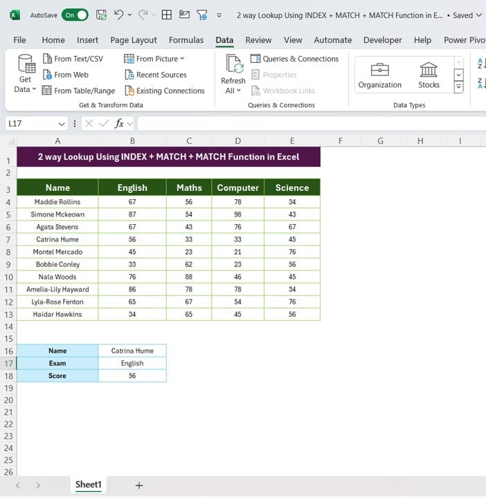
Step 1: Setting Up Your Data
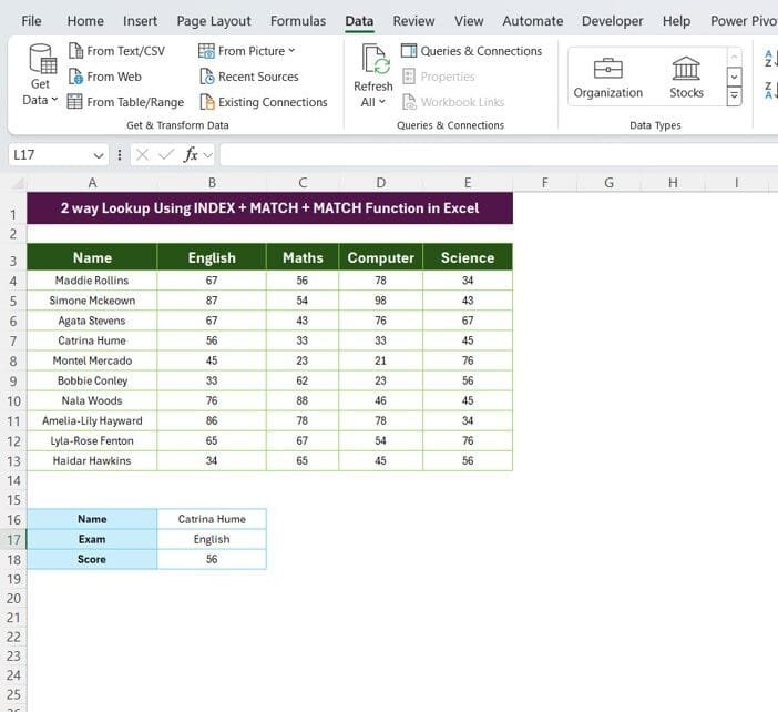
To start, you’ll need a table where you can use both row and column headers. For this example, let’s say you have a table of sales data for different products across several months. The rows will be your product names, and the columns will be the months.
Step 2: Using the INDEX Function
At the heart of this lookup is the INDEX + MATCH + MATCH Function in Excel. This function returns the value of a cell in a given range based on the row and column numbers you provide.
=INDEX (range, row number, column number)
Step 3: MATCH to Find the Row
Now, we’ll use the first MATCH function to figure out which row contains the product you’re looking for. The MATCH function finds the position of your search term within a range.
=MATCH (lookup value, lookup array, match type)
For instance, if you’re looking for “Product A” in your table’s row labels, the MATCH function will return the row number where it’s found.
Step 4: MATCH Again for the Column
Next, we use another MATCH function, this time to find the position of the month (or your column header). You’ll follow the same syntax, but this time apply it to your column labels.
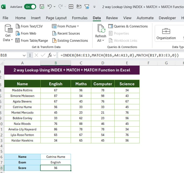
Step 5: Bringing It All Together
Finally, it’s time to combine these functions. The final formula will look something like this:
=INDEX(data range, MATCH(product, row labels, 0), MATCH(month, column labels, 0))
This formula will return the value at the intersection of your specified product and month.
Why You’ll Love This Method
More flexible than VLOOKUP or HLOOKUP – You’re not limited to just one direction.
Perfect for large datasets – Easily look up values no matter the complexity of your table.
Dynamic – You can update it for different values by changing your input cells.
Common Mistakes to Watch Out For
Even though this method is powerful, there are a few things that can trip you up:
- Mismatched Data: Make sure your row and column headers are the same as what’s in your formula, or Excel won’t find them.
- Range Selection: Be sure to select the correct ranges for your INDEX + MATCH + MATCH Function in Excel. This is crucial to getting accurate results!
Let’s Wrap This Up
By now, you’ve seen how powerful the INDEX + MATCH + MATCH Function in Excel combo can be for performing 2-way lookups in Excel. This method not only saves you time but also opens up more possibilities for analyzing data in both rows and columns. So, the next time you’re working on a dataset and need to perform a lookup, ditch VLOOKUP and try this instead!
Visit our YouTube channel to learn step-by-step video tutorials
Watch the step-by-step video tutorial:
Click hare to download the practice file