Looking for ways to find and retrieve data in Excel efficiently? Whether you’re managing a small dataset or working with hundreds of entries, Excel’s LOOKUP functions can save you time and effort. In this blog post, we’ll walk through four different 4 type of LOOKUP functions in Excel + MATCH, XLOOKUP, OFFSET + MATCH, and VLOOKUP + CHOOSE. By the end, you’ll know how to use each one to fetch data based on IDs, and you’ll be confident in applying these techniques to your own projects.
What Are LOOKUP Functions in Excel?
Before we dive into the examples, let’s quickly understand why LOOKUP functions are so valuable. These functions allow you to search for a value in one column and return the corresponding value from another column. This is especially useful when dealing with large tables where manually finding data could take forever.
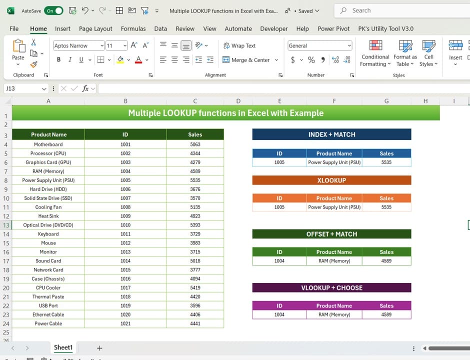
Now, let’s explore the data we’ll be using.
We’ll use the ID column to fetch the Product Name and Sales using different LOOKUP functions.
1. The Classic Combo: INDEX + MATCH

Let’s start with the INDEX + MATCH combo. It’s a flexible alternative to VLOOKUP and a fan favorites among Excel users.
Formula to Get Product Name:
=INDEX ($A: $A, MATCH ($E6, $B: $B, 0))
Formula to Get Sales:
=INDEX ($C: $C, MATCH ($E6, $B: $B, 0))
Example:
For ID 1005, this formula returns:
- Product Name: Power Supply Unit (PSU)
- Sales: 5535
Why Use INDEX + MATCH?
- You can search horizontally and vertically.
- It’s more flexible compared to VLOOKUP since the lookup value doesn’t need to be in the first column.
2. The Newbie Star: XLOOKUP

The XLOOKUP function is a newer addition to Excel, and it’s quickly becoming a go-to for many users. It simplifies the lookup process and offers more functionality than the older VLOOKUP.
Formula to Get Product Name:
=XLOOKUP (E11, B3:B24, A3:A24)
Formula to Get Sales:
=XLOOKUP (E11, B3:B24, C3:C24)
Example:
For ID 1005, XLOOKUP returns:
- Product Name: Power Supply Unit (PSU)
- Sales: 5535
Why Use XLOOKUP?
- No need to worry about whether your lookup value is in the first column.
- It’s straightforward and eliminates some of the limitations found in other lookup functions.
3. OFFSET + MATCH: The Powerful Pair
The OFFSET + MATCH combination offers flexibility similar to INDEX + MATCH but with the added ability to dynamically reference ranges.
Formula to Get Product Name:
=OFFSET ($A$3, MATCH ($E17, $B$4: $B$24, 0), 0)
Formula to Get Sales:
=OFFSET ($A$3, MATCH ($E17, $B$4: $B$24, 0), 2)
Example:
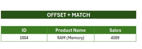
For ID 1004, the OFFSET + MATCH combo gives us:
- Product Name: RAM (Memory)
- Sales: 4589
Why Use OFFSET + MATCH?
- Great for dynamically changing data ranges.
- Allows more control over reference points in your dataset.
4. VLOOKUP + CHOOSE: The Versatile Option
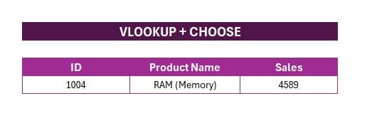
If you’re familiar with VLOOKUP, you’ll appreciate how the CHOOSE function can make it more powerful. This method allows you to lookup data from columns that are not adjacent.
Formula to Get Product Name:
=VLOOKUP (E23, CHOOSE ({1,2}, B4:B24, A4:A24), 2, 0)
Formula to Get Sales:
=VLOOKUP (E23, B3:C24, 2, 0)
Example:
For ID 1004, VLOOKUP + CHOOSE results in:
- Product Name: RAM (Memory)
- Sales: 4589
Why Use VLOOKUP + CHOOSE?
- It overcomes VLOOKUP’s limitation of needing the lookup value in the first column.
- Ideal for retrieving data from non-adjacent columns.
Conclusion
And there you have it! Four different ways to look up data in Excel using powerful functions. Each method has its strengths, whether you need flexibility, simplicity, or dynamic referencing. By mastering these LOOKUP functions, you can make your data work for you efficiently.
If you found this tutorial helpful, be sure to check out our YouTube video for a visual walkthrough of these functions!
Visit our YouTube channel to learn step-by-step video tutorials
Watch the step-by-step video tutorial:
Click hare to download the practice file

