Excel Magic Unleashed: A Step-by-Step Guide to Highlight Dates with Dropdowns
Welcome to a transformative journey into the world of Excel! In our latest video, “Excel Magic: Highlight Dates with Dropdowns & Conditional Formatting,” we’ve unlocked a powerful technique to enhance your data analysis skills. This easy-to-follow guide is perfect for both beginners and seasoned Excel users. Let’s dive in and turn your spreadsheets into a dynamic data display!
Step 1: Setting Up Your Data
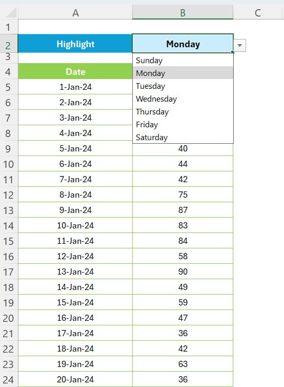
Imagine having a sales data sheet with dates in column A (A4:A24) and corresponding sales amounts in column B. Now, think about the power of highlighting specific rows based on the day of the week. Sounds intriguing, right? That’s exactly what we’re going to achieve!
Step 2: The Magic of Dropdown Lists
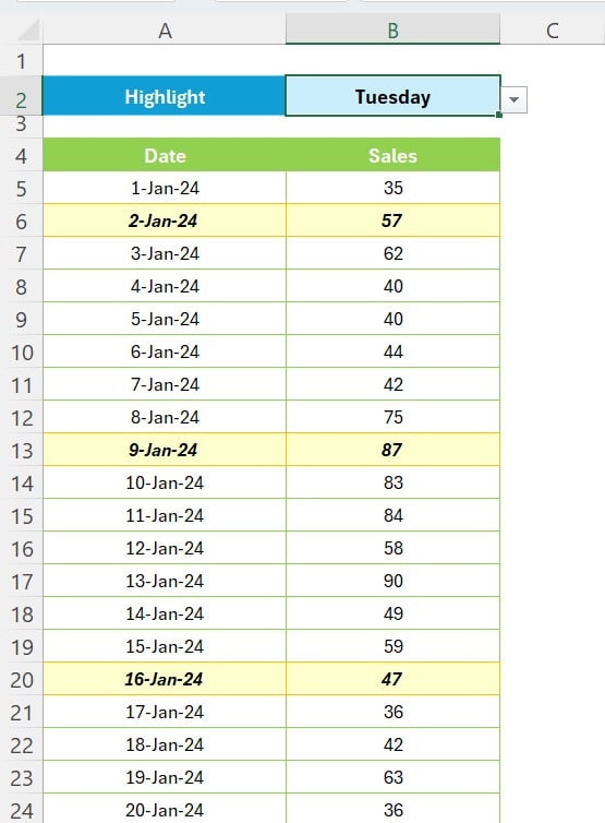
At the heart of our process is a simple yet effective dropdown list, positioned in cell B2, containing the days of the week: Sunday, Monday, Tuesday, Wednesday, Thursday, Friday, and Saturday. This dropdown is your control panel, steering the highlighting magic in your data.
Step 3: Initiating Conditional Formatting
Ready for some Excel wizardry? Here’s how we bring your data to life:
- Select Your Data Range: Click and drag to select the range A5:B34. This range is your canvas for the conditional formatting art.
- Accessing the Hidden Power of Excel: Press Alt+O+D shortcut key. This shortcut is your key to the “Conditional Formatting Rule Manager,” a gateway to endless possibilities.
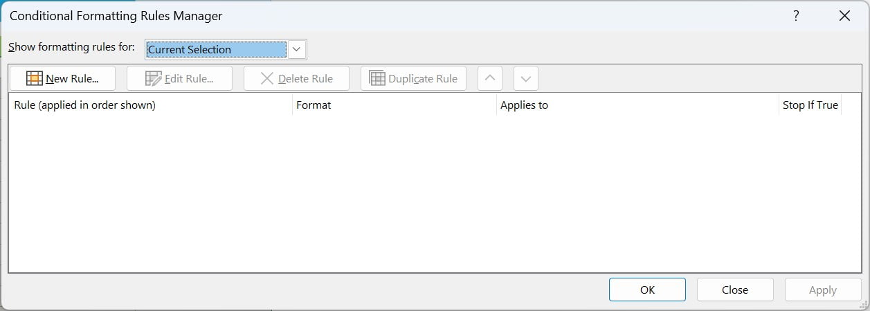
- Creating a New Rule: Click on ‘New Rule’ to open the “New Formatting Rule Window”. Here’s where the real magic begins.
- The Formula of Success: Choose “Use a formula to determine which cells to format”. This option allows you to customize how your data behaves.
- Crafting the Magic Spell: Enter the formula =TEXT($A5,”DDDD”)=$B$2. This formula is the heart of our operation, linking your dropdown selection to the data.
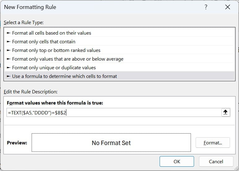
- Adding a Splash of Color: Click ‘Format’ to open the Format Cells window. Navigate to the Fill tab and choose a light yellow color. This visual cue will bring attention to your highlighted data.
- Defining Borders: Go to the Border tab, select a dark yellow color, and click ‘Outline’. This step adds clarity and emphasis to your highlighted data.
- Styling Your Data: Under the Font Tab, select ‘Bold Italic’ to make your highlighted data stand out even more.
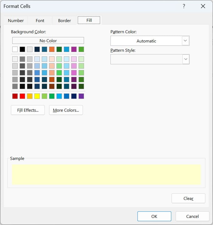
- Applying Your Settings: Click ‘OK’ and watch as your conditional formatting brings your data to life.
The Final Reveal: Excel Magic in Action
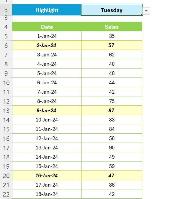
As you select different days from the dropdown, watch in awe as Excel dynamically highlights the rows corresponding to those days. This technique not only adds visual appeal to your data but also enhances your ability to analyze and interpret information quickly and effectively.
Conclusion: Your Journey to Excel Mastery
Congratulations! You’ve just elevated your Excel skills. This guide is more than just a tutorial; it’s your first step towards mastering dynamic data visualization in Excel. Remember, practice makes perfect, so experiment with different variations of this technique to suit your needs.
Ready to watch the magic unfold? Head over to our YouTube video here and witness the power of Excel in action. Happy Excel-ing!
Visit our YouTube channel to learn step-by-step video tutorials
