Do you need to calculate the average marks for students or any data set? Well, you’re in the right place! In this blog post, I’ll Walk you through a super easy way to find Average Marks with using Excel’s find Average Marks. You don’t need to be an Excel expert to follow along – it’s beginner-friendly and perfect for anyone.
Let’s dive in and get started!
Let’s Take a Look at the Data First
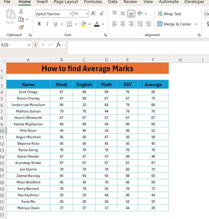
Before we begin with the actual calculation, let’s understand the data. Imagine you’re a teacher or student, and you have the scores of different students in four subjects: Hindi, English, Math, and SST (Social Studies). Now, the goal is to find Average Marks marks for each student across these subjects find Average Marks.
And so on. As you can see, we have the names of the students and their marks in four subjects, but we’re missing the average for each one That’s exactly what we’re going to calculate next! find Average Marks
What is the AVERAGE Function in Excel?
Now that we’ve got the data, let me explain how Excel’s AVERAGE function works. This function makes it incredibly easy to calculate the mean (or average) of a series of numbers. Whether you’re handling grades, financial data, or any other type of numbers, the AVERAGE function can be your best friend.
Here’s how the syntax looks:
=AVERAGE (number1, [number2], …)
In our case, “number1” and “number2” are the marks in the four subjects we want to calculate the average for.
How to Calculate Average Marks with Excel
Let’s move on to the fun part – using the find Average Marks to calculate the average marks for each student!
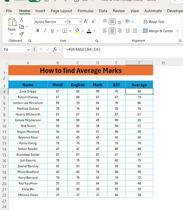
Let’s say we have the student marks in columns B to E (Hindi, English, Math, SST), and we want the average to appear in column F. To do this, simply enter the following formula in column F for the first student:
=AVERAGE (B4:E4)
This formula will calculate the average of Zack Ortega’s marks in Hindi, English, Math, and SST. Once you’ve done this, you can drag the formula down to apply it to all the other students as well. It’s that easy!
Step-by-Step Example
Let’s take an actual example to make this clearer. Zack Ortega has the following marks:
To find Zack’s average marks across these subjects, you would apply the formula:
=AVERAGE(B4:E4)
The result will be 80, which is Zack’s average score. Now, simply repeat this process for each student, and you’ll have all the averages ready in no time!
Why Use the AVERAGE Function?
You might be thinking, “Why should I use the AVERAGE function in Excel when I can just calculate it manually?” Well, let me tell you, there are several reasons:
- It’s Fast: No need to manually add and divide. Excel does all the heavy lifting for you in seconds.
- It’s Accurate: When you use a function like AVERAGE, you reduce the risk of making mistakes in your calculations.
- It’s Simple: You don’t need to be an Excel pro to use this function – it’s super easy to learn and apply!
The Result
Once you’ve applied the AVERAGE formula for all the students, your data will look something like this:
And just like that, you’ve calculated the average marks for each student in a matter of minutes!
Why the AVERAGE Function is Perfect for You
So, why is the AVERAGE function so helpful for tasks like these?
- Saves Time: You don’t need to manually calculate every average. With one formula, Excel takes care of everything.
- Prevents Errors: Manual calculations can lead to mistakes, but Excel eliminates that risk.
- Super Simple: Even if you’re new to Excel, you can use this function without any trouble.
Wrapping Up
There you have it! With just a few simple steps, you’ve learned how to find the average marks in Excel using the AVERAGE function. Whether you’re dealing with student scores or other data, this method is quick, easy, and accurate.
If you have any questions or need further clarification, feel free to drop a comment below! And don’t forget to check out our YouTube video for a visual walkthrough of this process.
Visit our YouTube channel to learn step-by-step video tutorials
View this post on Instagram
Click hare to download the practice file