If you’re looking to learn how to efficiently use the HLOOKUP formula in Excel, you’ve come to the right place! Whether you’re an Excel beginner or just want to improve your skills, this guide will walk you through the process, using a practical example. By the end of this blog post, you’ll understand not only what HLOOKUP FORMULA in Excel does but also how to apply it in real-life scenarios.
What is the HLOOKUP Formula in Excel?
Before we jump into the example, let’s quickly break down what HLOOKUP FORMULA in Excel is. The term stands for Horizontal Lookup, meaning it searches for a value in the first row of a range (or table) and returns a value in the same column from a row you specify.
It’s especially useful when your data is arranged horizontally, making it different from the more common VLOOKUP, which works with vertically aligned data.
Why Should You Learn HLOOKUP?
Now, you might wonder, “Why should I bother learning HLOOKUP?” Well, if you often work with large datasets that are organized in rows (instead of columns), then HLOOKUP is a must-know tool. It simplifies your workflow and allows you to quickly retrieve data without manually scrolling through long lists.
With that said, let’s dive into the example!
Example: Using HLOOKUP to Retrieve Grades
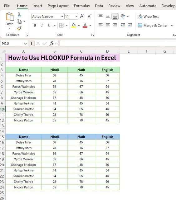
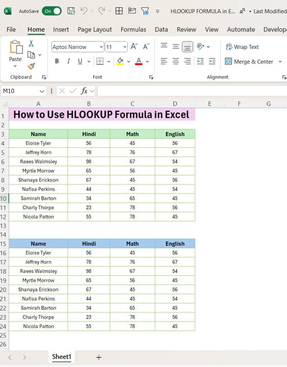
Imagine you’re managing a class of students, and you need to find their grades in different subjects: Hindi, Math, and English. Instead of manually searching for each student’s grade, you can use the HLOOKUP FORMULA in Excel to get the data instantly.
Step-by-Step Guide to Use HLOOKUP
Let’s say you want to quickly find the grade for Hindi for a specific student from this data set. Here’s how you can use the HLOOKUP formula:
- Choose your lookup value: In our case, we’ll use the subject (Hindi) as our lookup value.
- Select the table array: Our data range is from A3:D12. This includes the headers and all student information.
- Row index number: The row where you want to retrieve the data. In this case, for Hindi, it would be row 2.
- Range lookup: We want an exact match, so we’ll use FALSE.
Formula:
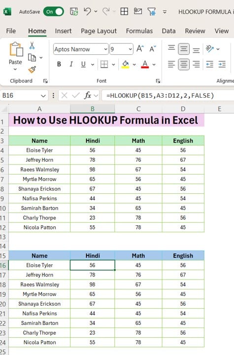
=HLOOKUP (“Hindi”, A3:D12, 2, FALSE)
Breaking Down the Formula
- “Hindi”: This is the value you’re searching for in the first row.
- A3: This is the table that contains the data you want to look through.
- 2: This tells Excel to return the value in the second row (in this case, Eloise Tyler’s Hindi grade).
- FALSE: This ensures we’re getting an exact match.
Output
After entering this formula, Excel will return the grade for Eloise Tyler in Hindi, which is 56.
You can repeat this formula for other students or subjects simply by adjusting the row index number or the subject you’re looking for.
More Examples
To get the Math grade for Raees Walmsley, you’d use the following formula:
=HLOOKUP (“Math”, A3:D12, 4, FALSE)
This would return 67, which is Raees Walmsley’s Math grade.
Why Use FALSE in the Formula?
You may have noticed we used FALSE at the end of our formula. This is to ensure that Excel only retrieves values with an exact match. If we used TRUE instead, it would return the nearest match, which is usually not what we want when dealing with precise data, like student grades.
Tips for Using HLOOKUP More Effectively
- Organize your data properly: HLOOKUP works best when your data is laid out clearly, with each category in a separate column and headers in the first row.
- Use with other formulas: HLOOKUP can be combined with other functions like IF to create more dynamic and powerful formulas.
- Avoid large datasets: While HLOOKUP is useful, it can be slow with large datasets. In such cases, consider using INDEX and MATCH for better performance.
Conclusion
And that’s how you use the HLOOKUP formula in Excel! As you can see, it’s a super handy tool for retrieving data from horizontally arranged datasets. Once you get the hang of it, you’ll wonder how you ever worked without it.
Ready to dive deeper? Watch our video on HLOOKUP Formula in Excel to see the formula in action and follow along with the example!
Visit our YouTube channel to learn step-by-step video tutorials
View this post on Instagram