Are you curious about what kind of data is hiding in your Excel cells? The TYPE Function in Excel with Examples is here to help! This function allows you to identify the exact type of data in any cell, which is incredibly useful for troubleshooting and improving your formulas. In this article, we’ll walk through how to use the TYPE function with some straightforward examples so you can start applying it right away. Let’s dive in!
Why Should You Use the TYPE Function?
Imagine you’re working on a spreadsheet with various data types—numbers, text, errors, and even logical values like TRUE and FALSE. The TYPE function makes it easy to identify what’s in each cell, so you don’t have to guess. Knowing the data type can prevent formula errors and ensure you’re working with the right kind of data, which means less frustration and more productivity!
The Syntax of the TYPE Function
Using the TYPE function is simple. Here’s the basic syntax:
=TYPE(value)
- Value: This is the cell or specific data you want to check.
After entering the formula, Excel will return a number that represents the data type:
1 – Numbers
2 – Text
4 – Logical values (TRUE or FALSE)
16 – Errors (like #DIV/0! or #VALUE!)
64 – Arrays (like {1,2,3})
Next, let’s see a clear example to better understand how this function works.
Example Dataset to Try the TYPE Function
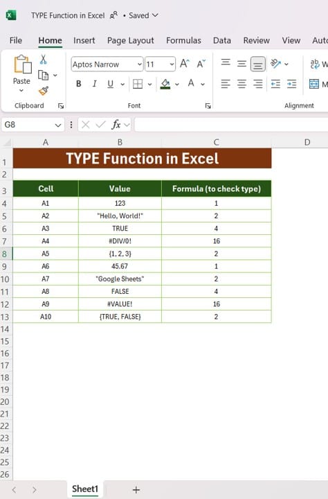
To illustrate how this function can help, we’ll use a sample dataset. Our data has three columns:
- Column A: Cell identifiers
- Column B: Data values (these include numbers, text, logical values, and errors)
- Column C: Results from using the TYPE function to identify each type
This table shows various data types and the results that the TYPE function returns for each. Now, let’s get practical and see how to apply the TYPE function step-by-step.
How to Use the TYPE Function in Excel (Step-by-Step)
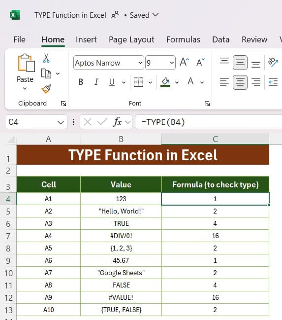
- Choose a cell where you want to apply the function. Let’s say you want to check the type of data in cell B4. Simply go to the cell in Column C next to it.
- Enter the formula for TYPE by typing =TYPE(B4) and press Enter.
- Observe the result. Excel will output a number in Column C that corresponds to the type of data in Column B. In this case, you’ll see a number like 1 for numeric values or 2 for text.
- Copy the formula down to analyze the entire column. By dragging the formula down from C4 to C13, you can instantly check the data types in each cell of Column B.
What Each Output Means
Let’s quickly recap what each number output from the TYPE function means:
1: Numeric values (e.g., 123, 45.67)
2: Text values (e.g., “Hello, World!”)
4: Logical values like TRUE or FALSE
16: Error values (e.g., #DIV/0!, #VALUE!)
64: Arrays (e.g., {1,2,3})
By understanding these types, you can decide how to handle each cell in your data, making your analysis more reliable.
Practical Ways to Use the TYPE Function
The TYPE function has some powerful applications beyond just identifying data types. Here are a few examples:
- Prevent Errors in Formulas: Knowing whether a cell contains an error or logical value can help you build error-proof formulas.
- Conditional Formatting: You can highlight cells with specific data types by combining the TYPE function with conditional formatting, making it easy to identify values that may need special attention.
- Data Validation: With TYPE, you can ensure that cells contain the expected data type before running calculations, which keeps your spreadsheet clean and accurate.
Example of Using TYPE in a Formula
Want to see the TYPE function in action? Here’s a quick example. To check the data type in cell B4, simply enter:
=TYPE(B4)
Once you press Enter, Excel will display a number that matches the data type. It’s that easy! You can repeat this process to analyze any cell’s data type.
Wrapping It All Up
The TYPE function in Excel is a handy tool that gives you an instant answer about what’s inside your cells. From text to numbers to errors, this function lets you identify and organize your data at a glance. With just a quick formula, you can understand your data better, prevent errors, and make smarter decisions on how to handle each cell.
Visit our YouTube channel to learn step-by-step video tutorials
View this post on Instagram
