Filter Function in Excel with Examples

Excel’s Filter Function in Excel is a game-changer when it comes to working with data. It enables you to quickly locate and display specific records based on your chosen criteria, making your data analysis faster and more precise. In this blog post, we’ll dive into how the FILTER function works in Excel and walk you through an example to help you get the hang of it. By the end, you’ll be filtering data like a pro Filter Function in Excel.

Table of Contents

Why Use the FILTER Function in Excel?

The Filter Function in Excel is incredibly helpful for displaying only the data you need without manually scrolling through long lists. This function can save time and minimize errors, especially when handling large datasets. Whether you’re tracking sales, analyzing performance metrics, or managing inventory, FILTER allows you to focus on relevant information, helping you make better decisions.

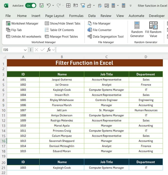
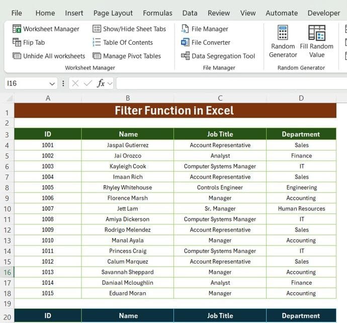
This data spans columns A through D and includes columns for ID, Name, Job Title, and Department, starting from row 3 to row 18.

The Goal

Our goal here is simple: filter this data to show specific records based on an ID. For example, let’s say we want to find the information for the employee with ID 1003, Kayleigh Cook. Instead of searching manually, we’ll use the FILTER function to extract only this record.

Step-by-Step Guide to Using the FILTER Function

Identify Your Range

In our example, the data is located in range B4

for the columns Name, Job Title, and Department. The ID column is located in A4

Enter the FILTER Formula

Now, to display data for a specific ID (let’s say ID 1003), we’ll enter the following formula in an empty cell:

=FILTER ($B$4: $D$18, $A$4:$A$18=A21)

Here’s what each part does:

$B$4: $D$18 specifies the range of data we want to display (Name, Job Title, and Department).
$A$4: $A$18=A21 checks for records where the ID in range A4

matches the value in cell A21 (where we’d enter the ID we’re looking for).

Key Tips for Using FILTER in Excel

Dynamic Filtering: As you update the value in A21 (or wherever you specify the ID), Excel will automatically adjust the output based on the new ID. This dynamic feature makes the FILTER function perfect for creating interactive reports.
Error Handling: If the FILTER function doesn’t find any matching results, it will display an error. To avoid this, you can add an error-handling option, like IFERROR, to display a custom message instead.

=IFERROR(FILTER($B$4:$D$18, $A$4:$A$18=A21), “No data found”)

Why the FILTER Function is a Must-Have

Using the FILTER function streamlines data analysis tasks, letting you zero in on the exact data you need with minimal hassle. Here are some quick benefits of using the FILTER function in Excel:

Timesaving: No need to manually search through rows; the function finds exactly what you need in seconds.
Error Reduction: Reduces the chance of manual errors by automating data extraction.
Dynamic Updates: Enables automatic updates when source data changes, making it ideal for real-time data analysis.

Try It Out!

The FILTER function can significantly enhance your efficiency when working with Excel. Give it a try on your dataset and see how quickly you can find specific information. Don’t forget to test it with various criteria to get comfortable with all the ways FILTER can work for you.

Visit our YouTube channel to learn step-by-step video tutorials

Youtube.com/@PKAnExcelExpert