Excel is a powerful tool for managing data, and the Excel, SUMIF formula in Excel tutorials is one of the essential tools that simplifies calculations by summing values based on specific conditions. In this post, we’ll walk you through the SUMIF formula, explore a practical example with detailed steps, and help you become more confident using this feature in Excel SUMIF formula in Excel.
What is the SUMIF Function in Excel?

The SUMIF function in Excel allows you to sum values in a range that meet specific criteria. This function is beneficial when working with data where you need totals based on a condition, such as summing sales for a particular product or totaling costs within a specific timeframe.
Example Scenario: Sales Data for Products
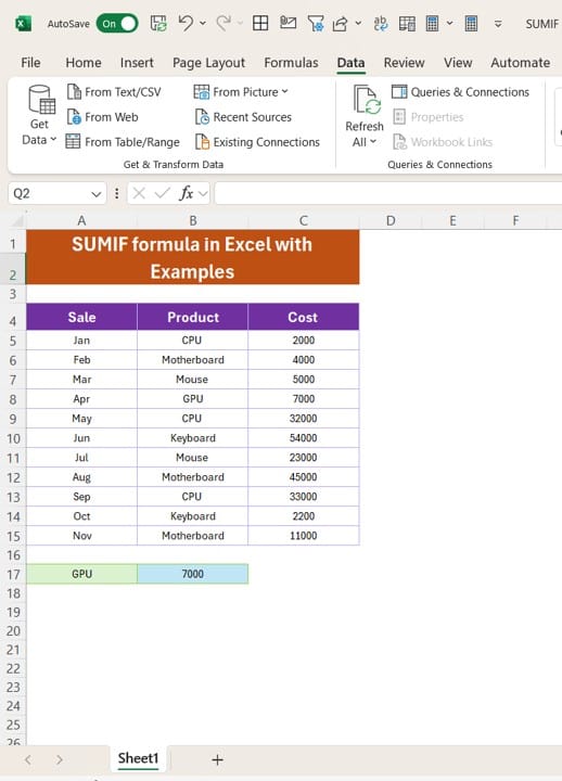
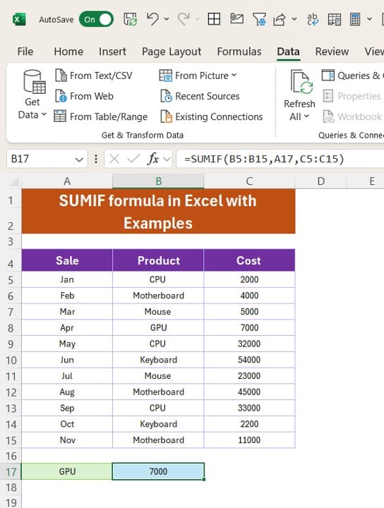
Let’s consider a scenario where we have sales data that includes months, products, and costs. Our goal is to calculate the total cost for each product type using the SUMIF function. Here’s a glimpse of the data we’ll be using:
Setting Up the SUMIF Formula

With our data ready, let’s set up the SUMIF function to calculate the total cost for a particular product. To use the SUMIF function, you’ll need three parameters:
- Range: The range where your criteria are located.
- Criteria: The condition that specifies which cells to sum.
- Sum_ range: The range of cells to sum if they meet the criteria.
For this example, let’s say we want to calculate the total cost for the product CPU. Here’s how we set up the SUMIF formula:
=SUMIF (B5:B15, “CPU”, C5:C15)
In this formula:
- B5 is the range where our products are listed.
- “CPU” is the criteria specifying that we only want to sum the costs where the product is CPU.
- C5is the range that contains the costs we want to sum.
When you input this formula into Excel, it will return the sum of all costs associated with the product CPU.
Step-by-Step Guide to Using SUMIF
- Identify the Column with Your Criteria: In this case, the Product column (B5) holds our criteria—specific product names.
- Define the Criteria: Type the name of the product you want to sum for (e.g., “CPU”).
- Select the Sum Range: Specify the column where the costs are listed (C5).
- Enter the Formula: Use the formula =SUMIF (B5:B15, “CPU”, C5:C15) and press Enter. Excel will calculate the sum of the costs where the product is CPU.
Output and Interpretation
After entering the formula, Excel provides the sum of costs for the product CPU, which you can find in the output cell. In our example, Excel will return the total cost for all entries where the product matches CPU.
Why Use SUMIF in Excel?
Using the SUMIF function has numerous benefits, especially for data analysis:
- Saves Time: Instead of manually summing values, SUMIF quickly calculates totals based on your conditions.
- Accuracy: Reduces the likelihood of errors by automating the sum calculations.
- Enhanced Data Analysis: Helps you drill down into data by filtering for specific criteria, making analysis more insightful.
Additional Tips for Using SUMIF
- Use Cell References for Criteria: Instead of typing the criteria directly into the formula, you can use a cell reference to make it easier to change the condition without editing the formula.
- Experiment with SUMIFS for Multiple Criteria: If you need to apply more than one condition (e.g., product and month), use the SUMIFS function, which supports multiple criteria.
Wrapping Up
The SUMIF function is a versatile tool that makes it easy to sum data based on specific conditions. By following this guide, you’re now equipped to use SUMIF to streamline your data calculations, making your work more efficient and your insights more valuable. Try applying this function to your own data and watch how Excel can transform your data analysis experience!
Visit our YouTube channel to learn step-by-step video tutorials
View this post on Instagram
Click hare to download the practice file


