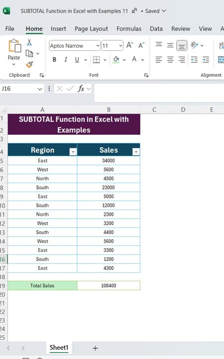
SUBTOTAL Function in Excel with Examples

Excel can do amazing things with your data, and the SUBTOTAL Function in Excel is one of the most useful tools for summarizing information without missing any key details. In this post, we’ll dive into how the SUBTOTAL function works, especially when you need to sum up specific parts of your data, like sales by region. Using our example data, I’ll walk you through how to use SUBTOTAL Function in Excel to get dynamic results SUBTOTAL Function in Excel.

Table of Contents

What Is the SUBTOTAL Function in Excel?

The SUBTOTAL function is versatile—it lets you calculate sums, averages, counts, and more, based on a set of values. But what makes it unique? Unlike regular functions, SUBTOTAL can automatically ignore hidden rows and filtered data, allowing for more flexible summaries.

Here’s a quick overview of its format:

=SUBTOTAL (function_ Num, ref1, [ref2], …)

function_ Num: A number from 1 to 11 (for including hidden rows) or 101 to 111 (for excluding hidden rows), each representing a different operation like sum, average, count, etc.
ref1, ref2…: The cell ranges you want to apply the subtotal function to.

Step-by-Step Solution with the SUBTOTAL Function

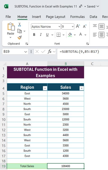
To calculate total sales in the Sales column (B4), we’ll use SUBTOTAL in Excel with the following formula:

=SUBTOTAL (9, B5:B17)

Here’s what each part of the formula does:

9 specifies the sum function.
B5 is the range of cells we want to sum.

Why Use SUBTOTAL Instead of SUM?

If you’re thinking, “Why not just use SUM(B5:B17)?”—that’s a great question! SUBTOTAL offers several advantages:

Excludes Hidden Rows: With SUBTOTAL, you can exclude any rows that have been hidden manually or through filters, keeping your summary clean and accurate for visible data only.
Multiple Operations: SUBTOTAL lets you do more than just sum. You can easily switch to other calculations by changing the function number.

This flexibility makes SUBTOTAL ideal for data that changes frequently or needs customized views based on filtered criteria.

Practical Example: Using SUBTOTAL for Filtered Data

Imagine you want to see sales totals for only certain regions, such as East and West. By applying a filter to the Region column, SUBTOTAL will update dynamically to show the sum for only the visible regions, without you having to adjust the formula.

Apply Filters to the data in your spreadsheet.
Select only the regions you want to view.
The SUBTOTAL function will automatically recalculate to reflect the visible rows only.

This is especially useful when you’re working with large datasets and need quick insights without modifying your formulas each time.

Changing the Function Type in SUBTOTAL

Want to find the average sales instead of the total? No problem! Change the function number from 9 (sum) to 1 (average):

=SUBTOTAL (1, B5:B17)

Now, you’ll get the average sales across the regions, again reflecting only visible rows if any rows are hidden or filtered.

Wrapping Up

The SUBTOTAL Function in Excel is a powerful tool for anyone working with Excel, particularly if you need dynamic summaries that adjust to filtered views. By using SUBTOTAL instead of more basic functions, you gain better control over your data, enabling more accurate reporting and analysis

Visit our YouTube channel to learn step-by-step video tutorials

Youtube.com/@PKAnExcelExpert