The INDEX function in Excel is an incredibly versatile tool that allows you to retrieve specific data from a table or range based on its row and column position. If you’ve been curious about how to simplify data extraction or enhance your Excel skills, this guide is for you!
In this blog post, we’ll walk you through how to use the INDEX function in Excel, complete with examples and step-by-step explanations. Whether you’re a beginner or an experienced Excel user, you’ll find actionable tips to improve your workflow. Let’s dive right in!
What is the INDEX Function in Excel?

The INDEX function returns the value of a cell within a specified range based on the row and column numbers you provide. It’s often used in combination with other functions like MATCH to create dynamic formulas.
Here’s the basic syntax:
INDEX (array, row _Num, [column Num])
- array: The range of cells or array where the data is located.
- row_ Num: The row number from which to retrieve data.
- column Num (optional): The column number from which to retrieve data.
How to Use the INDEX Function in Excel?

- Goal: Retrieve Specific Values Based on Row and Column Numbers
- Example 1: Fetching the Name of a Product
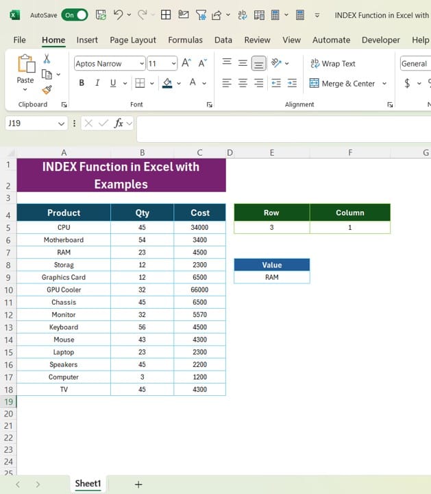
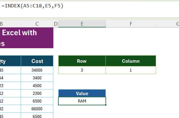
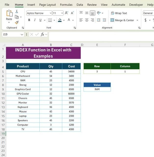
To retrieve the product in the 3rd row and 1st column of the data range, use the following formula:
=INDEX (A4:C18, 3, 1)
Steps:
- Select the cell where you want the result.
- Enter the formula =INDEX (A4:C18, 3, 1).
- Press Enter.
- Result: The formula returns RAM, as it’s the 3rd product in the list.
- Example 2: Fetching the Quantity
Let’s retrieve the quantity of the product in the 3rd row and 2nd column:
=INDEX (A4:C18, 3, 2)
The formula returns 23, which is the quantity associated with RAM.
Example 3: Fetching the Cost
Now, we’ll fetch the cost in the 3rd row and 3rd column:
=INDEX (A4:C18, 3, 3)
- Result: The formula returns 4500, which is the cost of RAM.
Using INDEX with the UNIQUE Function
You can enhance your Excel skills by combining the INDEX function with other powerful tools like UNIQUE. For instance, to extract a unique list of products from column A, use the formula:
=UNIQUE (A4:A18, FALSE, FALSE)
Steps:
- Select an empty range where you want the unique list to appear.
- Enter the formula above and press Enter.
- Result: You’ll get a unique list of all products in column A.
Why Should You Use the INDEX Function?
- Simplicity: Retrieve data effortlessly without complex logic.
- Efficiency: Works seamlessly with large datasets.
- Versatility: Can be combined with other functions for advanced operations.
Practical Use Cases for INDEX
- Automating reports by dynamically fetching values based on input criteria.
- Combining it with MATCH to create lookup formulas.
- Simplifying complex data extractions for dashboards.
Conclusion
The INDEX function is a must-know tool for anyone working with Excel. It not only simplifies data retrieval but also opens the door to creating dynamic and automated spreadsheets. With examples like these, you’re ready to incorporate the INDEX function into your daily tasks.
Visit our YouTube channel to learn step-by-step video tutorials
View this post on Instagram
Click hare to download the practice file


