A Chart for KPI Metrics
Moving Man Chart is very innovative chart to show the KPI Metrics like Service Level.

Below are the steps to create the Moving Man Chart in MS Excel
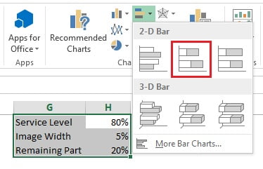
To create the moving man chart we need below support data:
- Service Level (or your Metric Name) and Service Level Performance(this cell will be changed with a formula later on)
- Image Width take as 5%
- Remaining Part – put formula =”100%-H1“

- Select Range “G1:H3” and go to Insert>>Charts>>2D Bar>> Insert Stacked Bar Chart
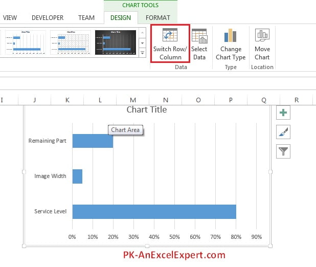
- Select the chart and go to Chart Tools>>Design Tab>>Click on Switch Row/Column
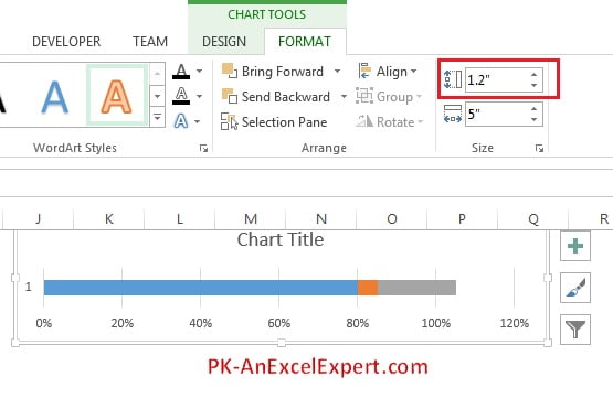
- Go to Format Tab and change chart height as 1.2″
- Remove the Chart Title, Gridlines, and Axes >> Primary Vertical

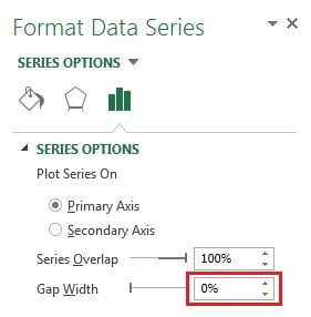
- Right Click on chart and click on Format Data Series
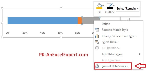
- In Series option take the Gap Width as 0%
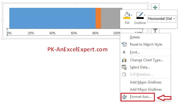
- Right Click on Horizontal Axis and click on Format Axis
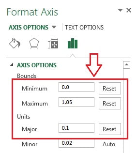
- Change the Axis option as below:
- Take Minimum as 0 (If it is already 0 then still change it so that it can be changed to Reset from Auto)
- Take Maximum as 1.05 (If it is already 1.05 then still change it so that it can be changed to Reset from Auto)
- Take Major as 0.1 (If it is already 0.1 then still change it so that it can be changed to Reset from Auto)
- Double click on the blue slice and fill color as No Fill
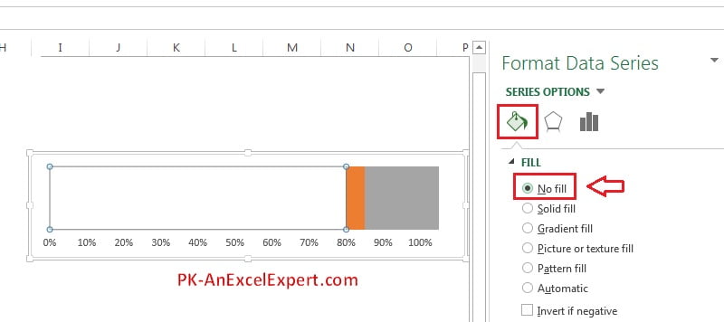
- Double click on the gray slice and fill color as No Fill
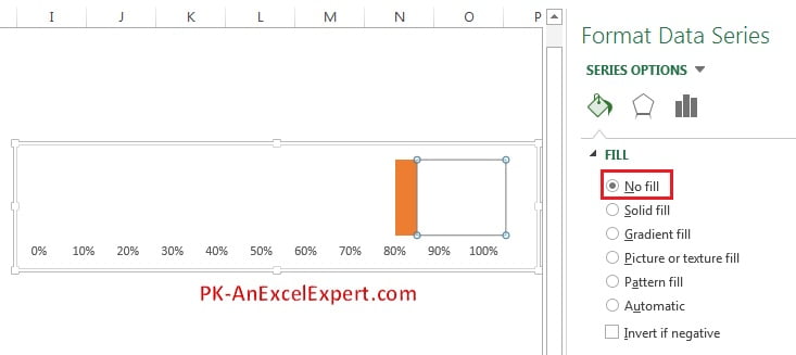
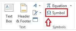
- Click on the worksheet anywhere and go to Insert>>Click on symbol
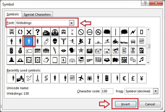
- In Symbol window select Font Webdings
- Scroll down and select Webdings-130 (A man icon)
- Click on Insert button
- Copy the cell wherein symbol was inserted.
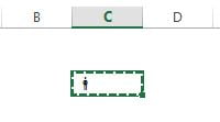
- Paste special as a picture.
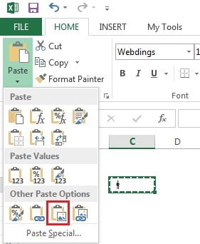
- Make the size of picture bigger as give below in the image.

- Select the Picture and go to Format>>Crop
- Crop the picture to remove the extra blank area.
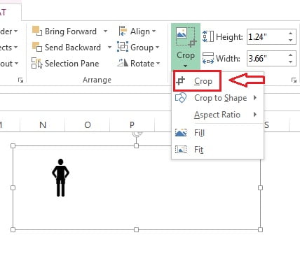
- Do not leave any extra are while cropping as given below image
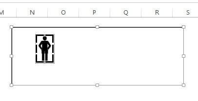
- After cropping successfully, copy the picture (Select the picture and press Ctrl + C)
- Select the orange slice in the chart and paste (press Ctrl + V)
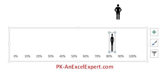
- Select the Chart area
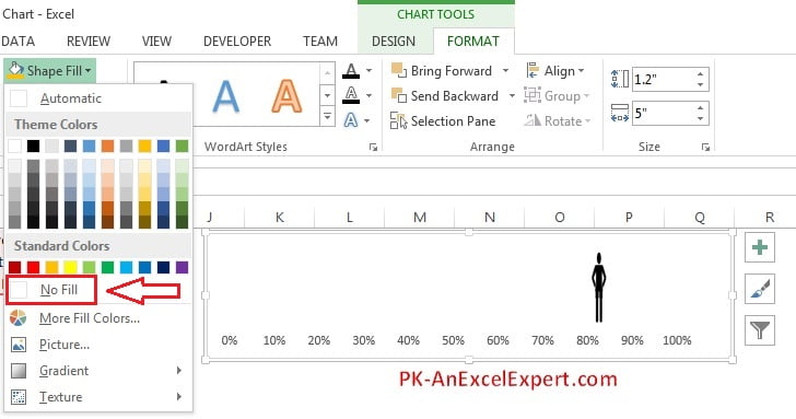
- Go to Format>>Shape Fill>>Fill as No Fill
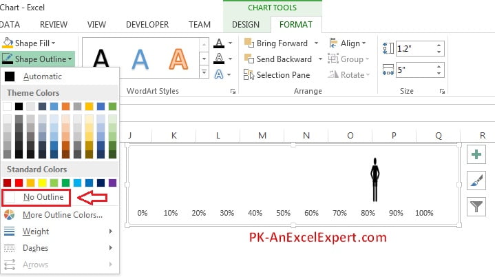
- Go to Format>>Shape Outline>>Select No Outline
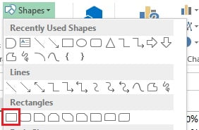
- Go to Insert>>Shapes>>Insert a Rectangle
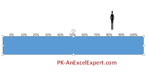
- Take the Rectangle width bigger than the chart width
- Right Click on the Shape and click on Format Shape
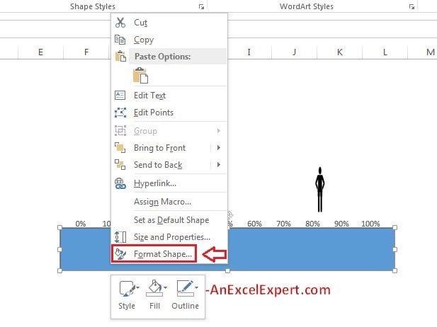
- Click on Effects button in Format Shape options
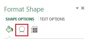
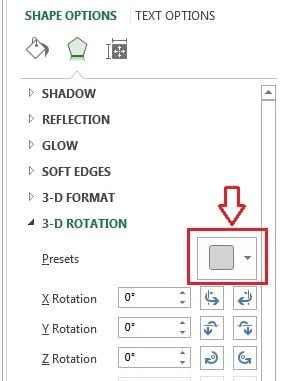
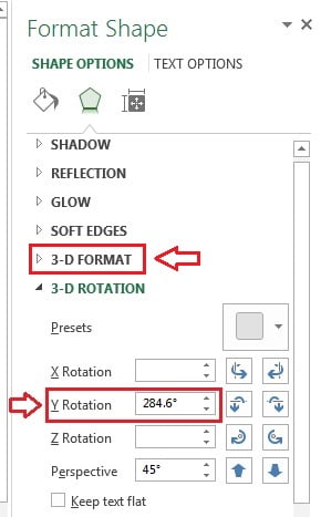
- Under 3-D Rotation, click on Presets
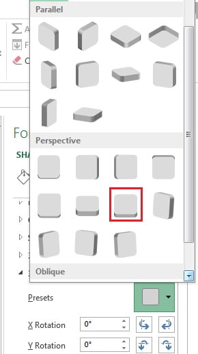
- Under the Perspective, select the Perspective Relaxed
- After Select the Perspective Relaxed Change the Y Rotation angle as 284.6°
- Click on 3-D Format Option.
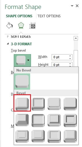
- In the 3-D Format option Select the Top bevel as Circle
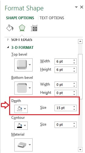
- Change the Depth as 15 pt
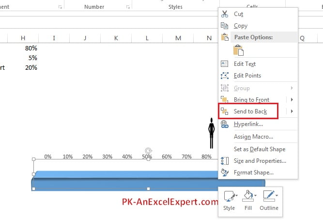
- Right click on the image and click on Send to Back
- Adjust the Image with the chart.
- Put your Active Service Level (Your Performance Metric) on range “F1”
- On Range “H1” Put formula (F1-2.5%)
Note: Since Image width has been taken 5%, hence the formula on range “H1” is “F1- half of Image Width” is being taken so that image will displayed on the chart in exact position.

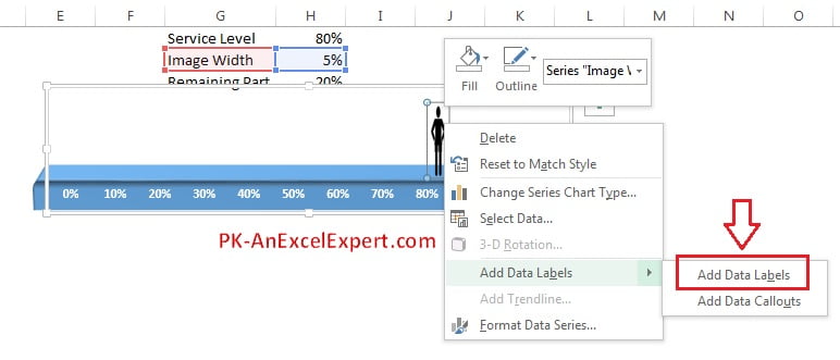
- Right click on the man image (in the chart)
- Click on the Add Data Labels
- Select the 5% (Data label on the chart)
- Go to formula bar and click on range “F1”
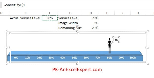
Our Moving Man Chart is ready.

Video Tutorial for The Moving Man Chart:
Visit our YouTube channel to learn step-by-step video tutorials