Are you managing multiple lists and need to find Check Common Names in Excel? Maybe you’re handling attendance lists, customer databases, or event attendees across different sessions, and you want to see who appears on both lists. In this blog post, we’ll walk through a simple, efficient method to Check Common Names in Excel. Using Excel’s FILTER and COUNTIF functions, we’ll quickly identify shared entries in two lists.
Ready? Let’s dive into the step-by-step guide!

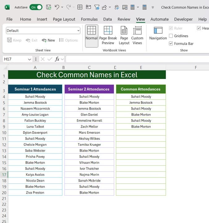
- Setting Up Your Data: We have entries with repeated names, as some individuals attended both seminars.
- Using COUNTIF to Check Common Entries: To identify the common names between these two lists, we’ll start by using the COUNTIF function. This function helps us count occurrences in a specified range, perfect for tracking names across both columns.
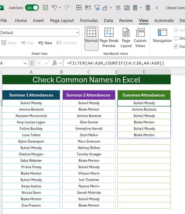
- Writing the Formula with FILTER and COUNTIF: To filter and display only the names that are common between the two columns, we’ll combine the FILTER and COUNTIF functions. Here’s the formula:
=FILTER (A4:A20, COUNTIF (B4:B20, A4:A20))
Breakdown of the Formula:
- COUNTIF (B4:B20, A4:A20) : This part checks each name in Column A against Column B and counts occurrences of each name. If the name appears in both columns, COUNTIF will register it as a match.
- FILTER (A4:A20, …) : This function then filters Column A based on the results from the COUNTIF function, displaying only those names that have at least one match in Column B.
These are the names that appear in both Seminar 1 and Seminar 2 attendance lists.
Using FILTER with COUNTIF is effective because:

- Simplicity: Instead of manually scanning and cross-referencing, you can instantly get results with this formula.
- Accuracy: This method ensures that every match, including duplicates, is captured accurately.
- Dynamic Updating: If your data changes, the formula will automatically adjust to include new entries or exclude removed ones.
Tips for Using This Method with Larger Data Sets
- Optimize with Named Ranges: If you’re working with larger datasets, consider using named ranges. This can make your formula more readable and manageable.
- Use Conditional Formatting: Want a visual approach? Try conditional formatting to highlight common names in both lists.
- Consider Removing Duplicates: If you only need unique Check Common Names in Excel, add a UNIQUE function around your FILTER result to remove duplicate entries.
Wrapping Up
And there you have it! With just a simple formula, we’ve identified Check Common Names in Excel between two columns in Excel. This method is not only efficient but also adaptable to various data types, making it a great tool for anyone who works with lists, registries, or databases.
Now it’s your turn to try it out! Let us know how it works for you, and if you have any tips to add, feel free to share. Happy filtering!
Visit our YouTube channel to learn step-by-step video tutorials
View this post on Instagram


