Color Scales option in Conditional formatting make very easy to visualize the values. It highlight the excel cells with different color on the base of their value.
Below are the steps to apply the Color Scales conditional formatting in an excel range-
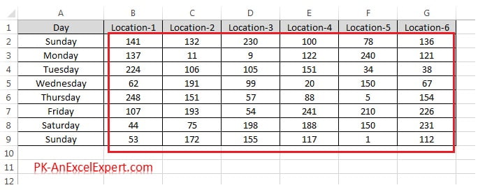
- Select the range on which you want to apply the Color Scales conditional formatting
- As in below image select “B2:G9”
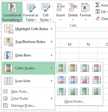
- Go to Home tab>>Conditional Formatting>>Colors Scales>>Choose a preset
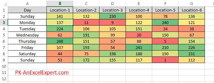
After applying the Color Scales preset your data will look like below image-
![]()
![]()