Today, we’re going to unravel the secrets of COUNTIF and SUMIF functions, and trust me, it’s going to be both fun and informative. Let’s dive right in and turn those Excel challenges into a piece of cake!
Let’s Begin with Our Data
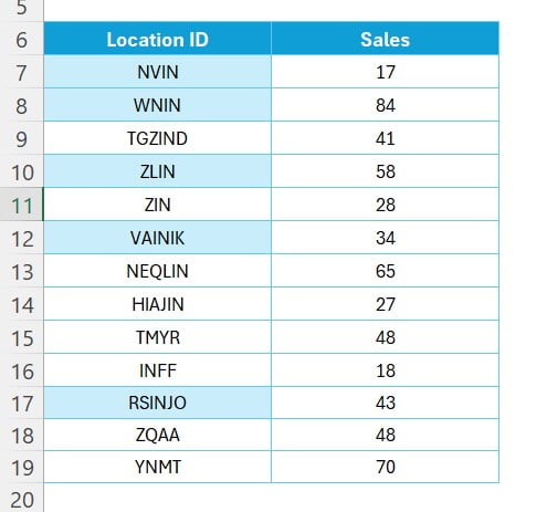
First things first, let’s set the stage with our data set. Imagine this: We have a bunch of Location IDs and Sales numbers sitting in our Excel sheet, waiting to tell us their story. Specifically, our Location IDs are in the range A7 to A19, and our Sales? They’re right next door, in B7 to B19. Here’s a glimpse of our data:

Discovering COUNTIF: A Simple Trick for Location IDs
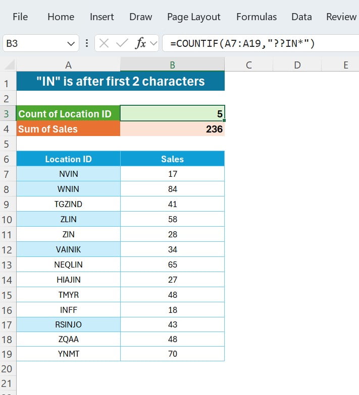
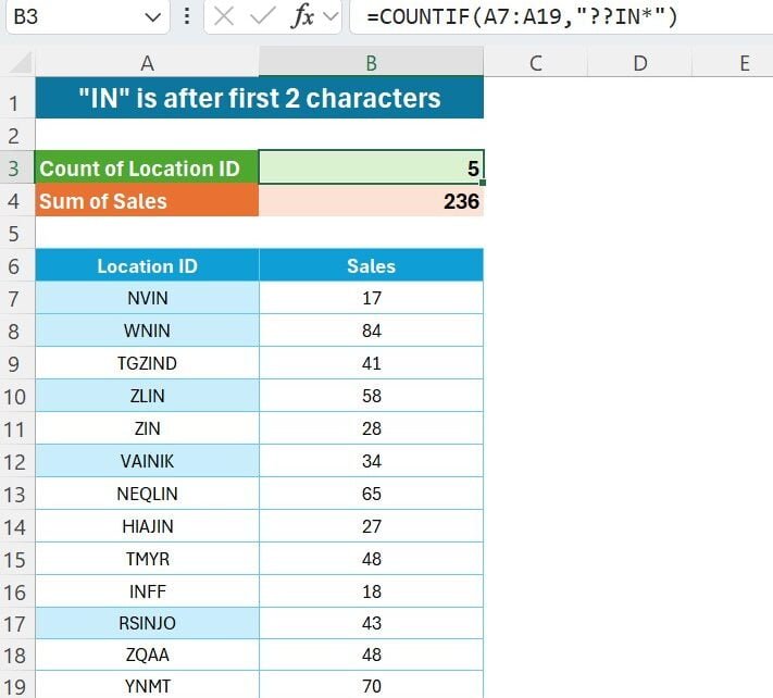
Now, let’s start with our first magical formula: COUNTIF. What’s our goal? Simply to count Location IDs where “IN” is snugly sitting after the first two characters. The magic spell we cast here is =COUNTIF(A7:A19,”??IN*”). Just like that, this formula does all the hard work and gives us the count. Easy-peasy, right?
The SUMIF: Summing Up Sales Effortlessly
Next up, we’re going to work our SUMIF magic. Our mission, should we choose to accept it, is to sum up the sales for those special Location IDs. And the magic formula? =SUMIF(A7:A19,”??IN*”,B7:B19). This little gem totals up all the sales for our specified IDs. It’s like Excel is doing a little happy dance for us!

Wrapping It Up: You’re Now an Excel Wizard!
And voilà! Just like that, you’ve added two powerful tricks to your Excel toolkit. Whether you’re just starting out or you’re an Excel old-timer, these tricks are sure to make your life easier.
Remember, Excel is not just a tool; it’s your secret weapon in making data tell its story. So go ahead, give these formulas a whirl on your data, and bask in the glory of your newfound Excel powers.
Visit our YouTube channel to learn step-by-step video tutorials


