Introduction
Welcome to a game-changing guide on how to revolutionize your Excel spreadsheets! Today, we’re diving into the world of dynamic, colorful progress bars in Excel cells. This method is not just visually appealing but incredibly functional, helping you track progress in a more intuitive way.
Learn Dynamic Colorful Progress Bars in Excel
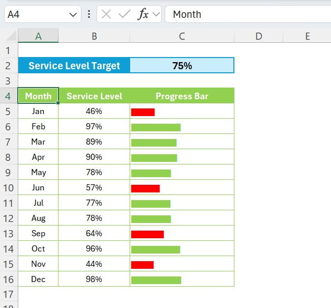
In this article, you’ll learn how to implement dynamic progress bars in Excel cells with color coding. This technique is perfect for visually representing data like service levels across different months. By the end of this guide, you’ll be able to create a progress bar that changes color based on whether the service level of a month meets the target.
The Data We Used
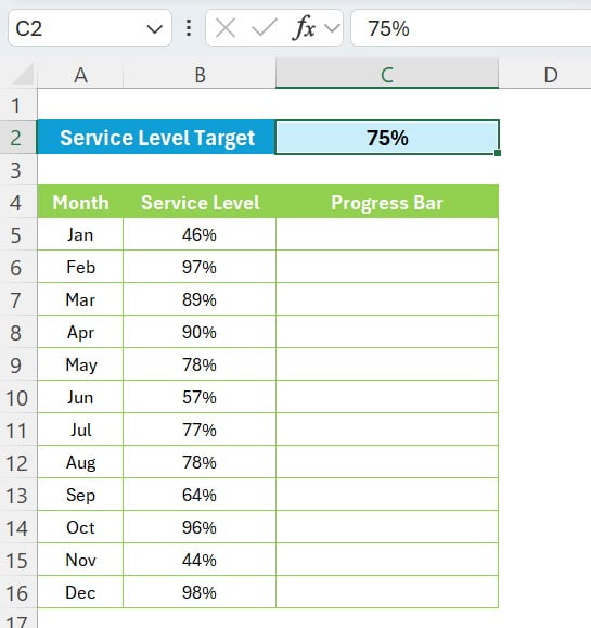
Here’s a brief overview of the data structure we used:
- In cell C2, we placed our Service Level Target.
- From A5 to A16, we listed the months from January to December.
- B5 to B16 contained the Service Level percentages for each corresponding month.
- In C5 to C16, we added the dynamic progress bar for each month’s Service Level.
Click to buy Dynamic Colorful Progress Bars in Excel cells
Step-by-Step Guide to Create Dynamic Progress Bars
Step 1: Setting Up the Foundation
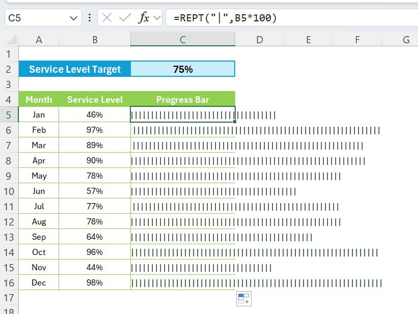
Firstly, input the formula =REPT(“|”,B5*100) in cell C5 and fill it down to C16. This formula creates the base for our progress bars.
Click to buy Dynamic Colorful Progress Bars in Excel cells
Step 2: Font Styling
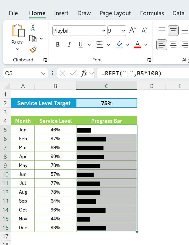
Change the font in the range C5 to C16 to “Playbill.” This font choice gives a bar-like appearance, crucial for our progress bars.
Click to buy Dynamic Colorful Progress Bars in Excel cells
Step 3: Initial Color Setting
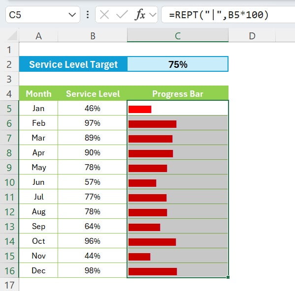
Set the font color for the range C5 to C16 as red. This will be our default color, indicating that the target hasn’t been met.
Click to buy Dynamic Colorful Progress Bars in Excel cells
Step 4: Conditional Formatting
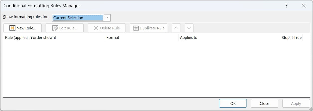
Press Alt+O+D shortcut key while selecting the range C5 to C16. This opens the Conditional Formatting Rule Manager.
Click to buy Dynamic Colorful Progress Bars in Excel cells
Step 5: Creating a New Rule
In the Rule Manager, click on ‘New Rule’ to bring up the New Formatting Rule window.
Step 6: Formula Selection
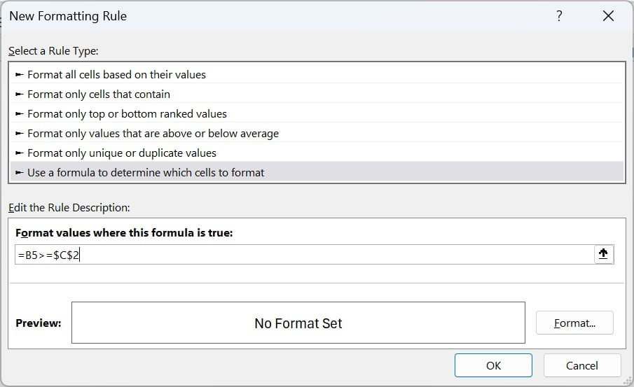
Choose “Use a Formula to determine which cells to format.” This option allows us to set conditions for formatting.
Step 7: Applying the Formula
Enter the formula =B5>=$C$2 in the formula box. This formula checks if the Service Level is meeting the target.
Click to buy Dynamic Colorful Progress Bars in Excel cells
Step 8: Formatting for Success
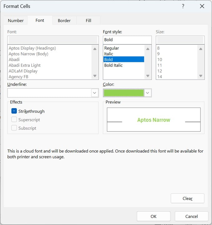
Click on ‘Format’ to open the Format Cells window, and select a green font color. Green will indicate that the target is met or exceeded.
Step 9: Finalizing the Format
Click ‘OK’ to apply the conditional formatting rule. Your progress bars will now dynamically change color based on performance!
Click to buy Dynamic Colorful Progress Bars in Excel cells
Conclusion: Your Excel, Supercharged!
Congratulations! You’ve successfully created dynamic, color-coded progress bars in Excel. This tool isn’t just about making your spreadsheets look better—it’s about making them work smarter. With these progress bars, tracking and presenting data becomes more efficient and impactful.
Remember, Excel is a powerful tool, and with tips like these, you can unlock its full potential. Keep experimenting, and don’t forget to share your progress bar creations with colleagues and friends!
Also see our other Progress Charts in Excel:
- Animated Progress Circle Chart
- How to WOW Your Boss: 3D Progress Circle in Excel
- Excel Magic: Stunning Animated Progress Circle Charts for Project Tracking
- Progress Circle Chart
Visit our YouTube channel to learn step-by-step video tutorials
Watch the step-by-step video tutorial:
Click to buy Dynamic Colorful Progress Bars in Excel cells
