Fill Blank Cells in Excel with the Value Above: 4 Quick Tricks

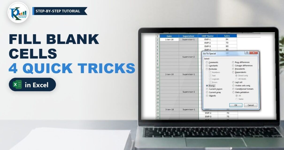
Need to fill blank cells in Excel with the value above? Exported reports often show a date or a supervisor name only on the first row of each group and leave the rest empty. That looks fine on screen, but pivot tables, filters, SUMIFS and dashboards need a value in every row. In this tutorial you learn PK’s four tricks to fill the blanks in seconds: a filter with Ctrl+D, Go To Special with Ctrl+Enter, an IF formula in a support column, and a five-line VBA macro. Download the practice file and follow along.

⬇️  Download the Fill Blanks Practice File
4 practice sheets, one per method · .xlsm (contains the Fill_Down macro) · Excel for Windows

Watch the Video Tutorial

In this six-minute video PK fills the Date and Supervisor columns four ways: filter plus Ctrl+D, Go To Special plus Ctrl+Enter, an IF support column, and a Fill_Down macro.

What You Will Learn

• Trick 1, Filter: show only the blank rows and fill them with one formula and Ctrl+D.
• Trick 2, Go To Special: select every blank cell at once and fill them all with Ctrl+Enter.
• Trick 3, Formula: build the complete column in a support column with IF, then paste it back as values.
• Trick 4, VBA: a tiny macro that fills any selected range in one click.
• Clean-up: fix dates that turn into numbers and convert formulas into values.

The Sample Data

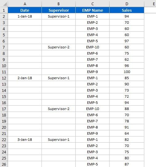
The practice file has the same data on four sheets, one for each method. There are four columns: Date, Supervisor, EMP Name and Sales, with 130 records in rows 2 to 131. Each date from 1-Jan-18 to 13-Jan-18 covers ten employees, but the date is typed only in the first row of the day (A2, A12, A22 and so on). The supervisor name appears only on the first row of each team: Supervisor-1 for EMP-1 to EMP-5 and Supervisor-2 for EMP-10 and EMP-6 to EMP-9.

For three or four groups you could select a value and press Ctrl+D, or copy and paste it down. For long data, use one of these tricks instead.

Trick 1: Fill Blank Cells in Excel Using a Filter

Step 1: Filter the blank cells

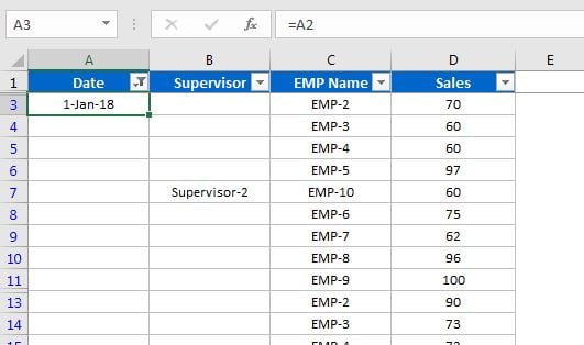
Click inside the data and turn on the filter (Data › Filter or Ctrl+Shift+L). Open the drop-down on the Date header, untick everything except (Blanks) and click OK. Only the empty date rows stay visible; in the video the status bar shows 117 of 130 records found.

Step 2: Enter one formula and fill it down

The first visible blank cell is A3. Type =A2 (the cell directly above it, even though row 2 is hidden by the filter) and press Enter. Now select from A3 down to the last visible row and press Ctrl+D. On a filtered range Excel fills only the visible cells, so every blank gets a formula that points to the row above it, while the original dates are left alone.

Step 3: Repeat for the Supervisor column

Clear the date filter, filter the Supervisor column to blanks, type =B2 in B3 and fill it down with Ctrl+D. Clear the filter and every row now shows the right date and supervisor.

Why it works: each formula refers to the cell above. The cell above is either an original value or another formula that already resolved to that value, so the value flows down until the next real entry starts a new group.

Trick 2: Select Blanks with Go To Special and Ctrl+Enter

This is the fastest manual method, and the one to remember.

Step 1: Select the range

Select both columns from the first data row to the end, here A2:B131.

Step 2: Select only the blank cells

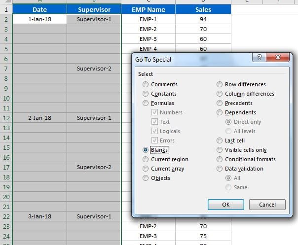
Press Ctrl+G (Go To), click Special, choose Blanks and click OK. Excel keeps the selection but drops every cell that has a value, so only the empty cells stay highlighted.

Step 3: Type one formula and press Ctrl+Enter

Without clicking anywhere else, type = and click the cell just above the active cell. If the active cell is B3, the formula is =B2. Now press Ctrl+Enter instead of Enter.

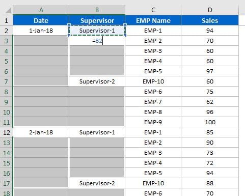
Why it works: Ctrl+Enter puts the entry into every selected cell. Because =B2 is a relative reference (it means the cell one row up), each blank cell gets its own version: A4 gets =A3, B8 gets =B7, and so on.

Step 4: Fix the date format

The new formulas in column A show numbers such as 43101 instead of dates, because the empty cells had the General format. Select column A and press Ctrl+Shift+3 to apply the date format.

Trick 3: Fill Blanks with an IF Formula in a Support Column

This method never touches the original data until you are happy with the result.

Step 1: Add the formulas

In the empty columns next to the data, enter:

• In E2: =IF(A2="",E1,A2)
• In F2: =IF(B2="",F1,B2)

Fill both formulas down to row 131.

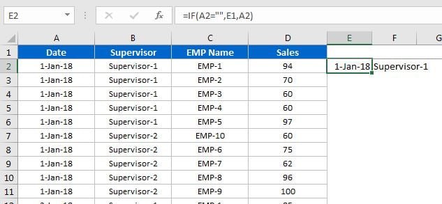
How the formula works

• A2="" tests whether the original cell is empty.
• If it is empty, the formula returns E1, the result of the support column one row up, which already holds the last value seen.
• If it is not empty, it returns A2 itself, so a new date or supervisor starts a new group.

Step 2: Paste back as values

Format column E as a date with Ctrl+Shift+3. Then copy E2:F131, select A2 and use Paste Special › Values. Columns A and B now hold the complete data as fixed values, and you can delete the support columns.

Trick 4: Fill Blank Cells Using VBA

Step 1: Add the macro

Press Alt+F11 (or Developer › Visual Basic), choose Insert › Module and paste this code:

Option Explicit

Sub Fill_Down()

Dim rng As Range

For Each rng In Selection
    If rng.Value = "" Then
        rng.FillDown
    End If
Next

End Sub

How the code works

• For Each rng In Selection visits every selected cell, row by row from top to bottom.
• If rng.Value = "" Then skips cells that already have a value.
• rng.FillDown on a single cell copies the cell above into it, just like pressing Ctrl+D. Because the loop runs top to bottom, the cell above is always filled already, so the value keeps flowing down the group.

Step 2: Run it

Select the range to fill, for example A2:B131, go to Developer › Macros, choose Fill_Down and click Run. The dates and supervisors are filled as values, with the formatting copied from the cell above, so no date fix is needed. Save the workbook as .xlsm to keep the macro.

Modern Alternatives (Addition)

These two options are additions to PK’s original four tricks.

Power Query Fill Down. If the same report arrives every week, load it with Data › From Table/Range, select the Date and Supervisor columns and choose Transform › Fill › Down. Power Query fills empty (null) cells with the value above, and the step repeats automatically on every refresh. See Fill values in a column (Microsoft Learn).

One-line VBA with SpecialCells. This version does Trick 2 in code: it selects the blanks, writes a formula that points one row up into all of them at once, and converts the result to values.

Sub Fill_Blanks_With_Value_Above()
    On Error Resume Next   'no blanks in the selection: do nothing
    Selection.SpecialCells(xlCellTypeBlanks).FormulaR1C1 = "=R[-1]C"
    On Error GoTo 0
    Selection.Value = Selection.Value   'turn the formulas into values
End Sub

Common Errors and Fixes

• Dates show as 43101 or similar. The filled cells use the General format. Select the column and press Ctrl+Shift+3.
• Values change after sorting. Tricks 1 and 2 leave formulas that point to the row above. Copy the columns and use Paste Special › Values before you sort or delete rows. (Addition.)
• No cells were found. Go To Special shows this when the selection has no truly empty cells. Cells that contain a space or an empty text from a formula are not blank; clear them first. (Addition.)
• The header is copied into row 2. The first data row was blank, so there was no value above it except the header. Always start the selection at a row that already has a value.

Tips

• Use Ctrl+Enter any time you want the same entry or formula in many selected cells, not just for blanks.
• In the filter method, select from the first visible blank to the last visible row before pressing Ctrl+D.
• Store the Fill_Down macro in your Personal Macro Workbook to use it in every file.
• Microsoft’s reference for the method behind Trick 4: Range.FillDown method (Microsoft Learn).

Want It Ready-Made?

For one-click clean-up shortcuts right in your ribbon, try the free PK’s Utility Tool in Excel VBA add-in, or browse more Excel utilities and converters on NextGenTemplates.com. To master IF, lookup and data-cleaning formulas step by step, join the video course Excel + AI Mastery: 100 Essential Formulas and Real-World Projects.

Related Tutorials

• Quick Data Formatting by Personal Macro
• Paste Special in Microsoft Excel
• 3 Flash Fill Tips in Excel
• 10 Super Useful Productivity Tips in Excel
• Absenteeism Report in Excel

Frequently Asked Questions

How do I fill blank cells with the value above in Excel?

Select the column range, press Ctrl+G, click Special, choose Blanks and click OK. Type an equals sign, click the cell just above the active cell and press Ctrl+Enter. Every blank cell now points to the cell above it.

What does Ctrl+Enter do in Excel?

It enters what you typed into every selected cell at once instead of only the active cell. With relative references, each cell gets its own adjusted formula, which is why one keystroke fills all the blanks correctly.

Why do my dates turn into numbers like 43101 after filling the blanks?

Excel stores dates as serial numbers. The new formulas in the blank cells take the General format, so they show the serial number. Select the column and press Ctrl+Shift+3 to apply a date format again.

Should I keep the formulas after filling the blanks?

Usually no. The formulas point to the cell above, so sorting or deleting rows can change the results. Copy the filled columns and use Paste Special, Values to turn them into fixed values.

Which method is best for large data?

Go To Special with Ctrl+Enter is the fastest manual method for any size of data. Use the VBA macro when you repeat the job often, and Power Query when the same report arrives every week.

Can I download the practice file?

Yes. The free workbook has one sheet for each of the four methods plus the Fill_Down macro. Use the green download button near the top of this page.

About the Author

PK is a Microsoft Excel expert and trainer and the founder of PK: An Excel Expert and NextGenTemplates.com. He has been teaching Excel, VBA, Power Query and Power BI since 2016 on his YouTube channel.

Conclusion

Now you can fill blank cells in Excel four ways: filter and Ctrl+D, Go To Special and Ctrl+Enter, an IF support column, or a short macro. For a one-time clean-up, Go To Special is the quickest; for a job you repeat, use the macro or Power Query. Whichever you pick, convert the result to values and fix the date format, and your data is ready for pivot tables, reports and Excel dashboards.