When working with data in Excel, extracting specific types of information—like text from a mixed list—can streamline analysis and organization. In this guide, we’ll dive into the powerful FILTER and ISTEXT Function in Excel. Together, they can help you filter out only text data from a mixed list of values, making it easier to focus on the information you need.
Let’s walk through how you can use the FILTER and ISTEXT Function in Excel step-by-step, including examples to help clarify their practical applications!
Why Use FILTER and ISTEXT in Excel?
Excel’s FIFILTER and ISTEXT Function in Excel allows you to filter out data based on specific criteria, while ISTEXT identifies whether a cell contains text. When combined, they become a powerful toolset for isolating text from a mixed set of data. Imagine a scenario where you have names mixed with numbers, and you want to extract only the names. This is exactly where these functions shine!
With just a simple formula, we can focus on text entries, leaving out any numeric or other types of data. Let’s see how it works.
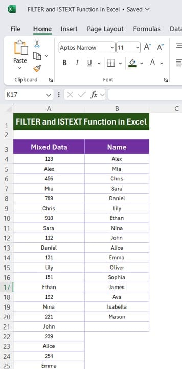
Data Setup for Our Example
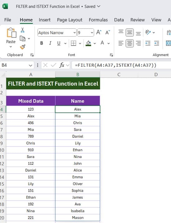
- To demonstrate the FILTER and ISTEXT functions, let’s consider the following dataset. We have two columns of data—Mixed Data in column A and Name in column B:
- Our goal is to extract only the text values from Column A (Mixed Data).
Step-by-Step Guide: Using FILTER and ISTEXT to Extract Text
- Understand the Formula: The formula we’ll use combines FILTER and ISTEXT as follows:
=FILTER (A3:A27, ISTEXT (A3:A27))
Here’s what each part does:
- FILTER (A3, …): This tells Excel to filter data within the range A3
- ISTEXT(A3): This acts as our criteria, specifying that we only want cells in range A3
that contain text.
Enter the Formula:
- Select a cell where you want your results to appear, such as cell C3.
- Type or paste the formula: =FILTER (A3:A27, ISTEXT (A3:A27))
- Press Enter to apply the formula.
- View the Results: Excel will automatically generate a list containing only the text values from the Mixed Data column.
As you can see, only the text values from the original data in Column A are displayed, with all numeric values filtered out.
Why This Combination Works
The ISTEXT function is a logical function that returns TRUE for cells containing text and FALSE for any other data types (like numbers). By wrapping this inside the FILTER function, we can tell Excel to include only the cells for which ISTEXT returns TRUE. This way, you can easily separate names or any text data from mixed data columns.
Practical Applications
You might wonder where else this technique could be helpful. Here are a few scenarios:
- Sorting Data for CRM Systems: Extract client names from lists where IDs and names are mixed.
- Contact Lists: Filter out only contact names when phone numbers and names are stored in a single column.
- Data Cleaning: Quickly isolate non-numeric data for cleanup or analysis.
Pro Tips for Working with FILTER and ISTEXT
- Adapt for Different Ranges: The formula can easily be modified to cover different ranges, so feel free to adjust as per your data structure.
- Use with Other Functions: Combine FILTER and ISTEXT with additional functions (like SORT or UNIQUE) for more refined results.
- Error Handling: If the formula doesn’t find any text data, it will return a #CALC! error. Use IFERROR around the formula to handle such cases gracefully.
Final Thoughts
The combination of FILTER and ISTEXT functions in Excel offers a simple yet effective solution for isolating text from mixed data columns. Whether you’re managing customer lists, organizing project data, or tidying up a data import, this dynamic duo of Excel functions can make your job easier FILTER and ISTEXT Function in Excel.
Visit our YouTube channel to learn step-by-step video tutorials
View this post on Instagram

