FILTER Data based is one of the most crucial tasks in Excel, especially when you want to narrow down results based on specific criteria—like a particular month. In this blog post, we’ll dive into how you can use the powerful FILTER function in Excel to extract data based on a specific month. Don’t worry, it’s simpler than it sounds, and by the end of this post, you’ll feel confident applying it in your own Excel sheets!
Understanding the FILTER Function in Excel
Before we get into the specifics, let’s quickly talk about the FILTER function. This function allows you to extract data from a larger dataset based on specific criteria. What makes it so valuable is that it dynamically adjusts when your data changes, meaning it will always show the correct filtered results without needing to update manually.
Why Filter by Month?
FILTER Data based by month can be extremely useful when dealing with sales reports, financial summaries, or any dataset that includes dates. For example, if you have a list of transactions spanning multiple months, but you only want to see those that happened in March, you can easily FILTER Data based them using the FILTER function along with the MONTH function in Excel.
Step-by-Step Example: Filtering Data for a Specific Month
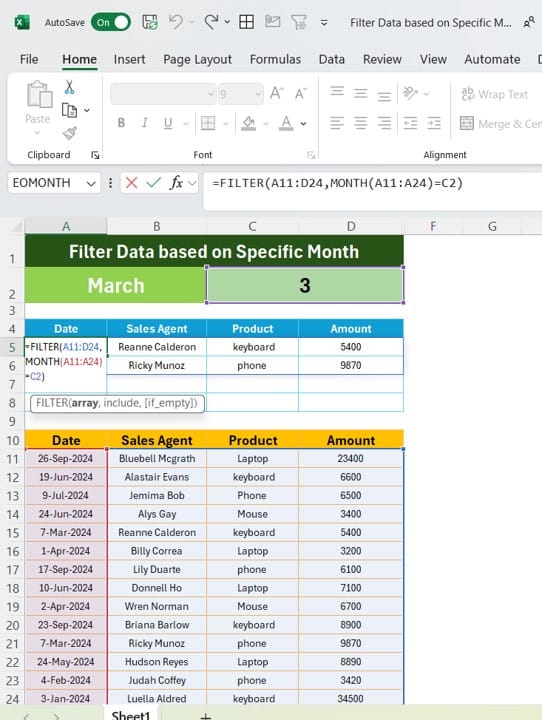
For this example, we have the following dataset:
- Date
- Sales Agent
- Product
- Amount
The Dataset
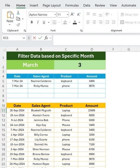
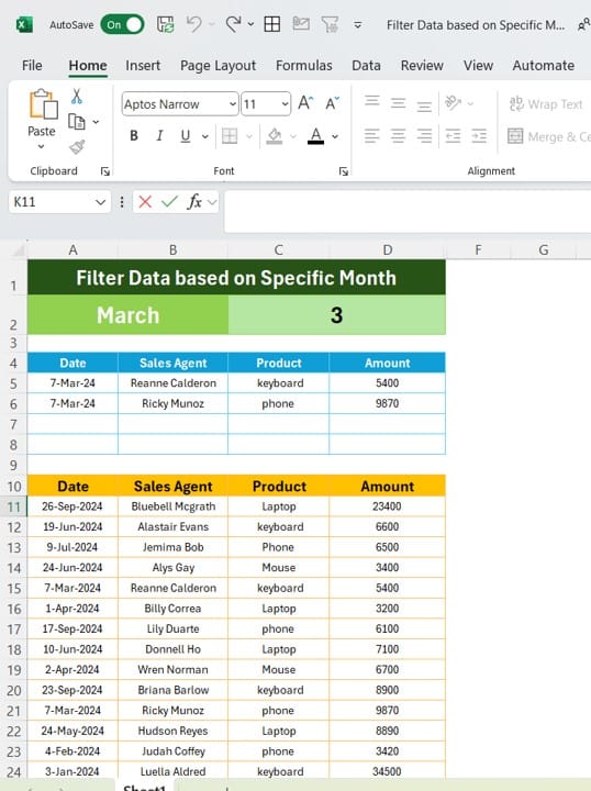
Our data ranges from A10, and it contains various transactions made by sales agents. Here’s a glimpse of the data:
The Goal
We want to FILTER Data based out the transactions that happened only in March.
Formula Breakdown
To FILTER Data based for March, we’ll use the following formula:
=FILTER (A11:D24, MONTH (A11:A24) = C2)
Here’s how it works:
- FILTER (A11): This is the range where we want to apply the filter.
- MONTH (A11) = C2: This checks if the month part of the date in column A is equal to the value in cell C2. In our example, cell C2 contains the number 3, which corresponds to March.
Applying the Formula
- Select a new area in your worksheet where you want the filtered data to appear.
- Enter the formula above.
- Voila! Excel will now display all the transactions from March in the new area you selected.
The Result
After applying the formula, you should see the following filtered data:
This output shows only the rows that match our criteria—transactions that occurred in March.
Why Use This Method?
Using the FILTER function in combination with MONTH has several benefits:
- Dynamic Updates: When new data is added, your filtered results update automatically—no need to adjust the filter manually.
- Quick Insights: Easily isolate the information you need from large datasets, whether it’s for reporting or analysis.
- Simple Yet Powerful: You don’t need to master complex formulas to get meaningful results.
Wrapping Up
Filtering data based on specific months in Excel is incredibly easy with the FILTER and MONTH functions. Not only does it save time, but it also makes data analysis smoother. Give it a try, and you’ll see how much more efficient your workflow becomes!
Visit our YouTube channel to learn step-by-step video tutorials
View this post on Instagram
Click hare to download the practice file
