Do you often find yourself wondering how to quickly identify Check Common Names between two list across different lists in Excel. Whether you’re comparing attendees for different seminars, members in various groups, or even products in multiple inventories, finding common elements can be crucial for effective data analysis.
Check Common Names between two list
In this post, we’ll walk you through a simple yet powerful method to check common names using the FILTER function combined with the COUNTIF function in Excel. By the end of this tutorial, you’ll be able to easily pinpoint common names between two or more lists with just a few clicks.
The Scenario: Comparing Seminar Attendees

Let’s say you’ve organized two seminars and want to find out which attendees participated in both. You have a list of attendees for Seminar 1 and Seminar 2, and now you need to identify the common attendees between these two events.
Example Data
Here’s what your data might look like:
Seminar 1 Attendees:
- Mohsin Mercado
- Patience Daugherty
- Jannat McGee
- Noel Hodson
- Keaton Millar
- Tilly-Mae Broughton
- Finn Mendez
- Om Randall
- Daphne McDonell
- Marcie Newman
- Jevon Hutchinson
- Krishan Whitley
- Haseeb Crawford
- Fitrat Hayward
- Ciaron Mackenzie
- Diesel Monroe
- Sammy-Jo Blankenship
Seminar 2 Attendees:
- Vikki Whittle
- Mujeeb Hood
- Patience Daugherty
- Orion Molina
- Keiron Lara
- Eduard Moran
- Krishan Whitley
- Kristy Beltran
- Harvie Ponce
- Aja Lowry
- Chyna Knowles
- Finn Mendez
- Vivienne Vasquez
- Sammy-Jo Blankenship
- Michael Golden
- Musa Glover
- Haseeb Crawford
With these lists, your goal is to figure out which names appear in both Seminar 1 and Seminar 2.
Step-by-Step Guide: Using FILTER and COUNTIF Functions
Here’s where the magic happens! We can use Excel’s powerful FILTER function in combination with the COUNTIF function to achieve our goal.
Set Up Your Data
Make sure your lists of attendees are organized in two separate columns. For example, Seminar 1 attendees in Column A and Seminar 2 attendees in Column B.
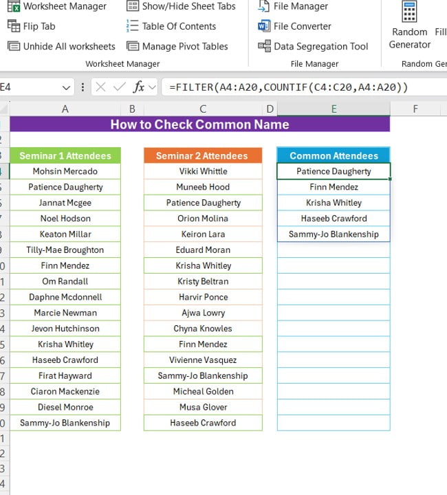
Write the Formula
In a new column, you’ll use the following formula to filter out the common names:
=FILTER (A4:A20, COUNTIF (C4:C20, A4:A20))
This formula works as follows:
- The COUNTIF function checks each name in Seminar 1 (Column A) against the list in Seminar 2 (Column B).
- The FILTER function then filters out only those names that appear in both lists.
Review the Results:
Once you enter the formula, Excel will display a list of names that are common between the two seminars.
The Result: Identifying Common Attendees
After applying the formula, you’ll see the list of common attendees like this:
Common Attendees:
- Patience Daugherty
- Finn Mendez
- Krishan Whitley
- Haseeb Crawford
- Sammy-Jo Blankenship
These are the individuals who attended both seminars, making it easy for you to follow up with them or analyses their engagement across events.
Why This Method Works
Using the FILTER and COUNTIF functions together is a quick and efficient way to compare lists in Excel. This approach can save you time, especially when dealing with large datasets. Plus, it ensures accuracy by eliminating the need to manually cross-check each name.
Final Thoughts:
Whether you’re managing events, tracking inventory, or analyzing data, Excel’s FILTER and COUNTIF functions are invaluable tools. By learning how to leverage them, you can streamline your workflow and make data comparison a breeze.
So, the next time you need to find common values between lists, give this method a try! If you found this tutorial helpful, be sure to check out our other Excel tips and tricks on our YouTube channel and blog. Happy Excel-Ing!
This structure ensures proper headings and subheadings, making the blog post more organized and SEO-friendly. It also maintains a conversational tone to engage your readers effectively.
Visit our YouTube channel to learn step-by-step video tutorials
View this post on Instagram