How to use HLOOKUP FORMULA in Excel

Have you ever wondered how to quickly search for data in Excel that’s arranged horizontally? Well, you’re in the right place because today, we’re diving into the HLOOKUP FORMULA in Excel a handy tool that makes looking up data across rows super simply! By the end of this guide, you’ll feel like an Excel pro, ready to use HLOOKUP FORMULA in Excel in your own spreadsheets.

Table of Contents

What is the HLOOKUP Formula?

The HLOOKUP (Horizontal Lookup) function in Excel allows you to search for a value in the first row of a table and return a value in the same column from another row. If you’ve used VLOOKUP before, this is similar but works horizontally, perfect when your data is structured across rows rather than down columns HLOOKUP FORMULA in Excel.

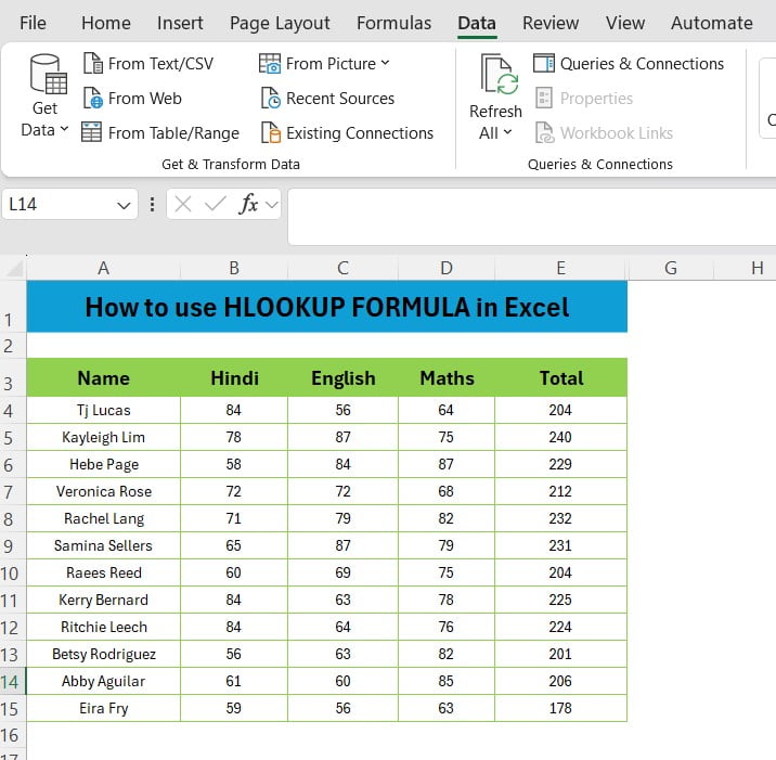
The Example Dataset

Let’s walk through an example so you can really see how this works in action. Here’s the data we’re using, arranged neatly in five columns:

This table includes student names, along with their marks in Hindi, English, and Math, and a Total column. Now, let’s say you want to quickly find Rachel Lang’s scores using HLOOKUP FORMULA in Excel.

How Does HLOOKUP Work in This Example?

The key idea here is to find Rachel Lang’s total scores using the HLOOKUP formula. We’ll be using the data in the range A3

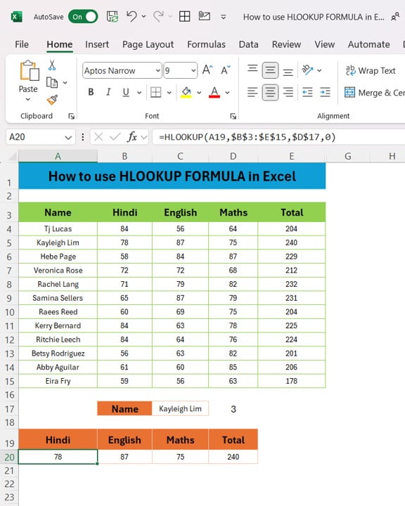
Formula:

=HLOOKUP(A19,$B$3:$E$15,$D$17,0)

Now, let’s break this down:

A18: This is the lookup value. In this case, it could be the name of the student you’re trying to find, such as “Rachel Lang.”
A3: This is the table array where you’re searching for the value. It includes the student names and their scores
6: This represents the row number where the result is found. Here, the row number is 6, which corresponds to the “Total” row.
FALSE: This tells Excel to find an exact match.

What Happens Next?

Once you hit enter, Excel will return Rachel Lang’s total score, which is 232. Amazing, right? You’ve just performed a horizontal lookup!

Why Should You Use HLOOKUP?

Now that you know how to use the HLOOKUP formula, you might wonder why and when it’s helpful. Here are a few reasons:

Perfect for Horizontally Arranged Data: If your data is laid out in rows instead of columns, HLOOKUP saves you time.
Quick and Precise: With just one formula, you can quickly find exact data matches.
Works in Various Scenarios: From student scores to financial data, HLOOKUP can be used in countless situations.

Wrapping Up

Now that you’ve learned how easy it is to use HLOOKUP, why not try it out in your own spreadsheets? Whether you’re looking up grades, sales data, or anything else arranged horizontally, this formula can make your life a whole lot easier HLOOKUP FORMULA in Excel.

Visit our YouTube channel to learn step-by-step video tutorials

Youtube.com/@PKAnExcelExpert