In this blog post, we’ll explore how to use the INT function in Excel, specifically for calculating age using dates. If you’ve ever wondered how to efficiently calculate the age of a person based on their date of birth, this article is for you! By the end, you’ll have a clear understanding of the INT function in Excel and how to use it effectively in Excel with real-world data.
Understanding the INT Function in Excel
The INT function in Excel is used to round down a number to the nearest integer. In simpler terms, it chops off any decimal places, leaving you with a whole number. This is super handy when dealing with age calculations because we want whole years, not fractions of years.
Syntax:
INT (number)
- number: This is the value you want to round down.
Now, let’s see this in action with an example!
- The Scenario: Age Calculation
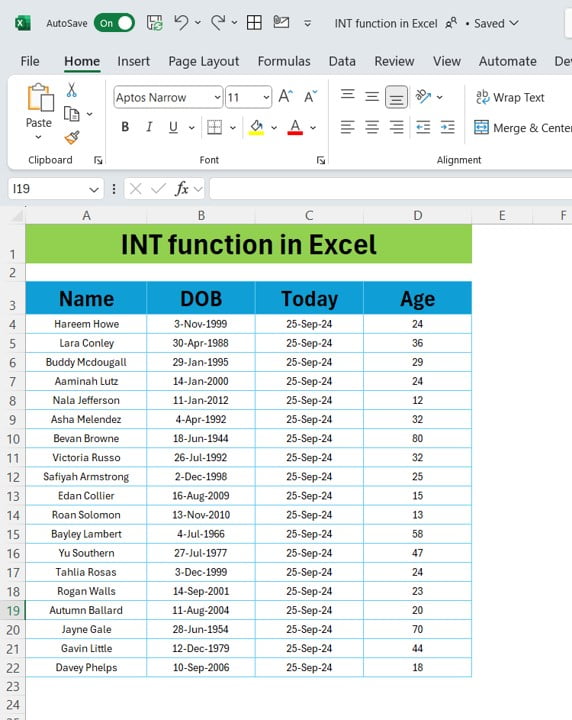
We have a list of employees, along with their Date of Birth (DOB), and we want to calculate their current age as of today’s date using Excel. The INT function will help us simplify this task. Below is the data we’ll be working with:
This table contains four columns:
- Name: The employee’s name.
- DOB: The employee’s date of birth.
- Today: The current date (set as 25th September 2024 for our example).
- Age: This is what we’ll calculate using the INT function!
The Formula: Calculating Age with INT Function
To calculate the age of each employee, we’ll subtract their date of birth from today’s date and divide the result by 365.25 (this accounts for leap years). Finally, we’ll use the INT function to round the result down to the nearest whole number.
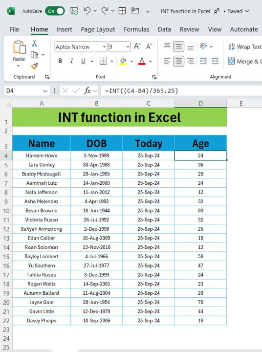
Here’s the formula we’ll use:
=INT((C4-B4)/365.25)
In this formula:
- C4: Refers to the cell containing today’s date.
- B4: Refers to the employee’s date of birth.
- 365.25: Divides the result by the average length of a year, including leap years.
- INT: Ensures the result is a whole number, representing the employee’s age.
Step-by-Step: Applying the INT Function
- Select the cell where you want to display the age. Let’s say you want the age to appear in column D, starting from row 4 (D4).
- Enter the formula:
=INT((C4-B4)/365.25)
Press Enter, and you’ll see the calculated age for that employee.
- Drag the formula down through the rest of the column to apply it to all employees.
That’s it! The INT function, combined with date calculations, will give you the exact age for each employee, just like in our example.
Why Use INT for Age Calculation?
The INT function is simple but powerful when it comes to working with whole numbers. In this case, it ensures that we don’t end up with partial ages (like 24.7 years) and keeps everything clean and accurate. The formula also accounts for leap years, thanks to the 365.25 divisor, which makes it more precise than just using 365 days.
Final Thoughts
Now that you know how to use the INT function in Excel for age calculation, you can easily apply it to your own data. Whether it’s for employee records, student data, or personal projects, this simple formula can save you a lot of time and effort!
If you found this tutorial helpful, feel free to share it with your friends and colleagues. And if you have any questions, drop them in the comments below – we’re always happy to help!
Visit our YouTube channel to learn step-by-step video tutorials
View this post on Instagram

