If you’re working with large datasets in Excel, you’ve probably encountered situations where you need to look up values based on more than one criterion. The XLOOKUP function is a powerful tool that can help you do just that. In this blog post, we’ll walk you through how to use XLOOKUP with multiple criteria to make your data analysis smoother and more efficient.
Whether you’re an Excel novice or a seasoned pro, this guide will break down the process step by step, making it easy to follow along. So, let’s dive right in!
Understanding the Scenario
Imagine you’re managing sales data for various products sold both online and offline, in different packet sizes. You need to find the sales figure for a specific combination of product, packet size, and sales channel. This is where XLOOKUP with multiple criteria comes into play.
The Data
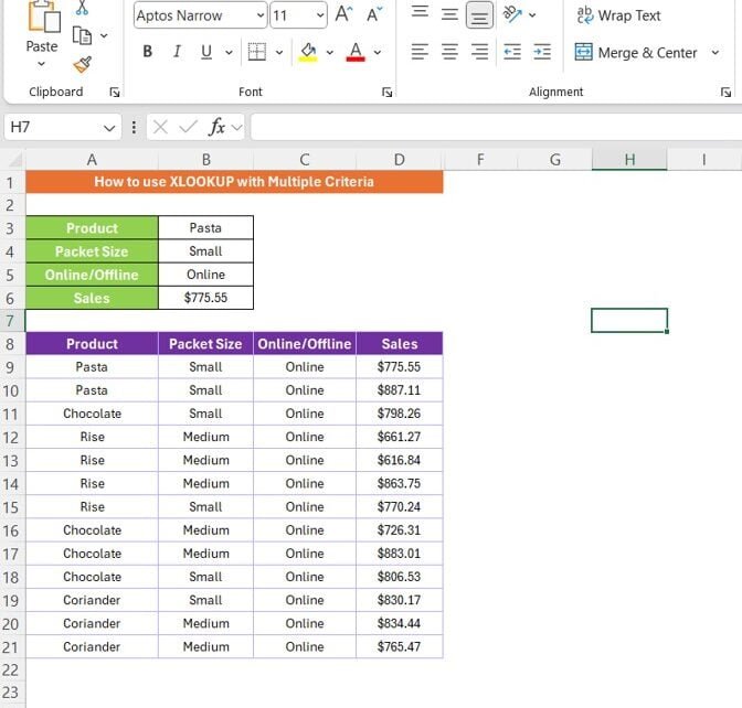
We have the following data, split across four columns:
- Product (Range: A8)
- Packet Size (Range: B8)
- Online/Offline (Range: C8)
- Sales (Range: D8)
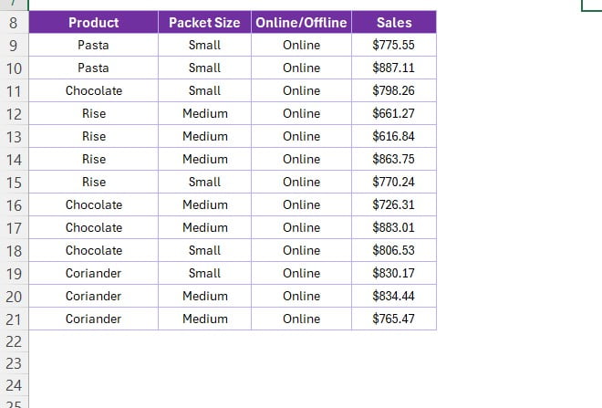
As you can see, we have sales data for different products sold in various packet sizes across online platforms. Now, let’s move on to how you can use XLOOKUP to retrieve specific data based on multiple criteria.
Crafting the XLOOKUP Formula
To look up a specific sales figure, we’ll use the XLOOKUP function, which is incredibly versatile and efficient, especially when dealing with multiple criteria.
Here’s the formula we’ll use:
=XLOOKUP(B3&B4&B5, A8:A21&B8:B21&C8:C21, D8:D21)
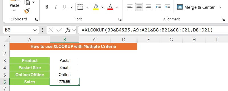
Breaking Down the Formula:
- B3&B4&B5: This part of the formula combines the values from the cells B3 (Product), B4 (Packet Size), and B5 (Online/Offline) into a single string. This string acts as our lookup value.
- A8:A21&B8:B21&C8:C21: This combines the ranges for Product, Packet Size, and Online/Offline into a single array, which XLOOKUP will search through.
- D8:D21: This is the return array, meaning that once XLOOKUP finds the matching string in the combined array, it will return the corresponding value from this range.
Example Scenario:
Let’s say you want to find the sales figure for a “Small” packet of “Pasta” sold “Online.” Here’s how you’d set up your input cells:
- Product (B3): Pasta
- Packet Size (B4): Small
- Online/Offline (B5): Online
When you enter the formula into a cell, Excel will return the sales figure for that specific combination—in this case, ₹775.55.
Why Use XLOOKUP with Multiple Criteria?
You might be wondering, why bother with XLOOKUP when there are other lookup functions like VLOOKUP or INDEX-MATCH? The answer lies in its flexibility and efficiency.
- Flexibility: XLOOKUP allows you to search for values both horizontally and vertically, making it a one-stop solution for most lookup needs.
- Efficiency: With XLOOKUP, you don’t need to sort your data or worry about whether your lookup column is on the left or right. It just works!
Conclusion:
Using XLOOKUP with multiple criteria can save you a ton of time and headaches, especially when working with complex datasets. It’s straightforward once you get the hang of it, and the results speak for themselves. Now that you’ve learned how to use this powerful function, why not try it out on your own data?
Remember, practice makes perfect! So, open up Excel, input your data, and start using XLOOKUP to streamline your workflow today.
If you found this guide helpful, don’t forget to check out our YouTube video for a visual walkthrough. And as always, feel free to leave your questions or comments below—we’re here to help!
Visit our YouTube channel to learn step-by-step video tutorials
