Have you ever encountered those frustrating #N/A errors while working in Excel? You’re not alone! Excel’s IFNA Function in Excel is a fantastic tool to help handle these errors gracefully. With IFNA, you can catch #N/A errors and replace them with a custom message, like “Not Exist,” to keep your data clean and user-friendly. In this post, we’ll dive into the basics of the IFNA Function in Excel, explore how it works, and see practical examples that make it easy to use.
What is the IFNA Function?

The IFNA function in Excel checks for #N/A errors in a formula and lets you replace the error with a value of your choice. This function is particularly useful when performing lookups, calculations, or any tasks that might result in #N/A errors. The syntax for IFNA is simple:
=IFNA (value, Valentia)
- value: The formula or cell you want to check.
- Valentia: The value to display if an #N/A error occurs.
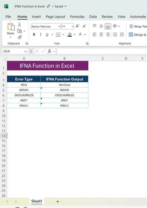
We’ll use the IFNA Function in Excel to catch any #N/A errors in the “Error Type” column (range A3) and replace them with “Not Exist” in the “IFNA Function Output” column (range B3). This helps ensure that your data looks neat and conveys the message you want, without unnecessary error messages.
Using the IFNA Function in Excel

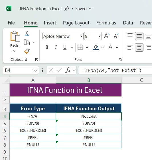
In our example, we want to handle the #N/A errors in Column A and display “Not Exist” when an #N/A error is encountered. To do this, we use the following formula in cell B4:
=IFNA (A4, “Not Exist”)
This formula checks the content of cell A4:
- If A4 contains an #N/A error, the formula returns “Not Exist.”
- If there’s no #N/A error, it simply returns the original value in A4.
Example Walkthrough: Step-by-Step
Let’s break down how this formula works with each type of error in our sample data:
- In cell B3: The value in A3 is #N/A. The formula =IFNA (A3, “Not Exist”) detects this error and displays “Not Exist” in B3.
- In cell B4: The value in A4 is #DIV/0! which is a different type of error. Since the IFNA function only catches #N/A errors, it leaves #DIV/0! as-is in B4.
- In cell B5: The value in A5 is “EXCELHURDLES” (no error). IFNA doesn’t make any changes and simply displays “EXCELHURDLES” in B5.
- In cell B6: The value in A6 is #REF! another type of error. Like with #DIV/0! IFNA doesn’t handle this, so #REF! appears in B6.
- In cell B7: The value in A7 is #NULL! Again, IFNA doesn’t affect this error type, so it remains #NULL! in B7.
This simple example demonstrates the versatility of the IFNA function, especially when dealing with data prone to #N/A errors.
Why Use IFNA?
Using IFNA helps make your spreadsheets more professional and readable by:
- Preventing Error Disruption: IFNA catches errors like #N/A, allowing you to display custom messages instead.
- Enhancing Data Presentation: Your data looks cleaner, as users won’t see confusing error messages.
- Providing Context: Replacing errors with specific messages (like “Not Exist”) gives users a clearer understanding of the data.
Final Thoughts on the IFNA Function
The IFNA Function in Excel is a quick and effective solution to handle #N/A errors in Excel, especially when working with lookups or data validations that may return these errors. By catching these errors, you ensure your data appears organized and informative.
Now that you know how to use IFNA, try applying it to your own data! Whether you’re working on a large dataset or a simple spreadsheet, IFNA is a handy function that makes your data look clean and professional.
Visit our YouTube channel to learn step-by-step video tutorials
View this post on Instagram
Click hare to download the practice file


