Microsoft Excel has always been an indispensable tool for data manipulation and analysis. You can combine the data with the help of VStack and HStack functions in Excel. VStack and HStack help you to easily combine multiple arrays by stacking them vertically or horizontally, respectively. In this this article, we will provide you a comprehensive guide on using VStack and HStack functions in Excel, including their syntax, examples, and tips to handle various scenarios.
Understanding VStack and HStack Functions in Excel
1.1 VStack Function
The VStack function is used to combine the multiple arrays of the same number of columns into a single array by stacking them vertically. This is particularly useful when you need to consolidate data from various sources or tables with similar structures.
Syntax: =VSTACK(array1,[array2],...)
Here, array refers to the arrays (cell ranges) you want to append.
1.2 HStack Function
The HStack function, on the other hand, combines multiple arrays of the same number of rows into a single array by stacking them horizontally. It is quite useful while you need to merge data that is organized in a side-by-side format.
Syntax: =HSTACK(array1,[array2],...)
Here, array refers to the arrays (cell ranges) you want to append.
Practical Examples of VStack and HStack Functions in Excel
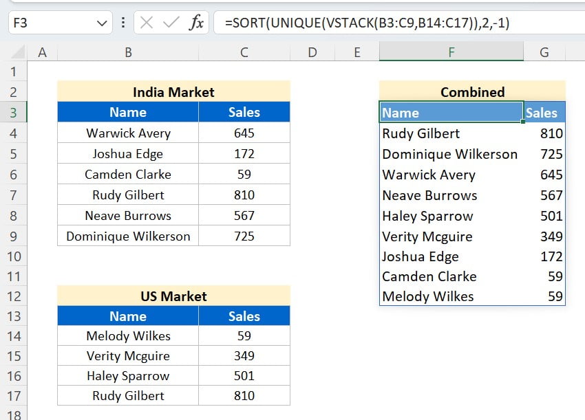
2.1 Combining Arrays with VStack
Example 1: Simple VStack
Imagine you have two tables with the same number of columns, and you want to stack them vertically. Then you can use below formula-
=VSTACK(A1:C4, A6:C9)
This formula will combine the data from A1:C4 and A6:C9 into a single array.
Example 2: VStack with Headers
To include column headers in the stacked array, simply reference an array containing the labels:
=VSTACK(A1:C1, A2:C4, A6:C9)
In this example, the column headers in A1:C1 are included in the resulting array.
2.2 Combining Arrays with HStack
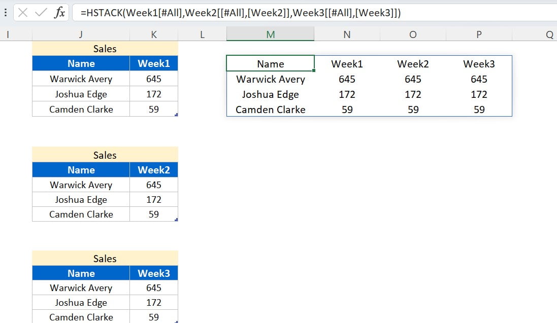
Example 3: Simple HStack
Consider two tables with the same number of rows that you wish to combine horizontally. The formula for this would be:
=HSTACK(A1:C4, E1:G4)
This will combine the data from A1:C4 and E1:G4 into a single array.
Example 4: HStack with Blank Columns
To include a blank column between the two groups of data, use the following formula:
=HSTACK(A1:C4, "", E1:G4)
In this example, an empty column will be inserted between the combined data.
Advanced Techniques with VStack and HStack Functions in Excel
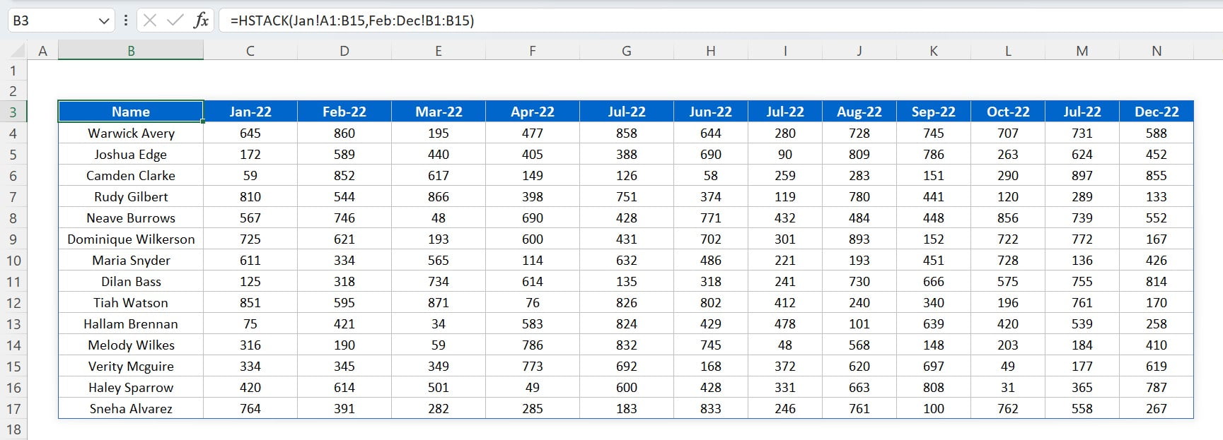
3.1 Combining Data from Multiple Sheets (3D Reference)
VStack and HStack functions can also be used to stack data spread across multiple sheets:
=HSTACK(Jan!A1:B15,Feb:Dec!B1:B15)
This formula will stack data from the range A1:B15 from sheet Jan to Dec.
3.2 Sorting Stacked Data
You can sort the combined data using the SORT function:
=VSTACK(SORT(A1:C4), SORT(A6:C9))
This formula will stack the data from A1:C4 and A6:C9 after sorting each range individually.

3.3 Filtering Data
Use the FILTER function to exclude specific rows or columns from the stacked data:
=VSTACK(FILTER(A1:C4, A1:A4="Criteria"), FILTER(A6:C9, A6:A9="Criteria"))
This formula will stack data from A1:C4 and A6:C9, only including rows where the criteria in column A are met.
Handling Errors
4.1 Mismatched Array Sizes
VStack and HStack functions require that the arrays being combined have the same number of columns or rows, respectively. If the arrays don’t match in size, you’ll encounter an error. To handle this issue, you can add or remove columns or rows as needed, or use the IFERROR function to return an alternative result.
Example:
=IFERROR(VSTACK(A1:C4, A6:C10), "Array size mismatch")
This formula will display the message “Array size mismatch” if there is a size mismatch between the arrays A1:C4 and A6:C10.
4.2 Nonexistent Sheets or Ranges
Using VStack or HStack with a nonexistent sheet or range will result in an error. To avoid this, ensure the sheet names and ranges in your formula are accurate. You can also use the IFERROR function to provide an alternative result.
Example:
=IFERROR(VSTACK('Sheet1:Sheet3'!A1:C10), "Invalid sheet or range")
This formula will display the message “Invalid sheet or range” if any sheet or range in the formula doesn’t exist.
Use Cases and Applications
5.1 Data Consolidation
VStack and HStack functions are particularly useful in consolidating data from multiple sources, such as sales reports, financial statements, or survey results, allowing for more efficient analysis and decision-making.
5.2 Reporting and Dashboards
You can use VStack and HStack functions to combine data from different tables or worksheets, making it easier to create summary reports, dashboards, and interactive charts.
5.3 Data Cleaning and Transformation
VStack and HStack functions can be combined with other Excel functions like SORT, FILTER, and UNIQUE to clean and transform data, making it ready for analysis, visualization, or importing into other software.
Conclusion
The VStack and HStack functions in Excel provide a powerful means to manipulate data by stacking arrays vertically and horizontally. These functions offer great flexibility, allowing users to combine data from multiple sources, sort and filter combined data, and handle errors effectively. By mastering the VStack and HStack functions, you’ll be well-equipped to handle a wide range of data manipulation tasks in Excel, making your work more efficient and accurate.
Frequently Asked Questions (FAQs)
Q. What are the VStack and HStack functions in Excel?
A. The VStack and HStack functions are Excel functions that allow you to combine multiple arrays (ranges of cells) vertically and horizontally, respectively. VStack stacks arrays on top of each other, while HStack stacks them side by side.
Q. Can I use VStack and HStack with different sized arrays?
A. VStack and HStack functions require that the arrays being combined have the same number of columns or rows, respectively. If the arrays don’t match in size, you’ll encounter an error. To handle this issue, you can add or remove columns or rows as needed, or use the IFERROR function to return an alternative result.
Q. How do I use the VStack and HStack functions in Excel?
A. To use the VStack and HStack functions in Excel, follow these steps:
- Type “=VSTACK(” or “=HSTACK(” in a cell where you want the combined data to appear.
- Select the arrays you want to combine, separated by commas.
- Close the parentheses and press Enter.
Example for VStack: =VSTACK(A1:B3, A5:B7)
Example for HStack: =HSTACK(A1:C3, D1:F3)
Q. Can I use VStack and HStack with data from different worksheets?
A. Yes, you can use VStack and HStack with data from different worksheets. To do so, include the worksheet name followed by an exclamation mark (!) before the cell range in your formula.
Example: =VSTACK(Sheet1!A1:B3, Sheet2!A1:B3)
Q. Can I combine VStack and HStack in the same formula?
A. Yes, you can combine VStack and HStack in the same formula to stack arrays both vertically and horizontally.
Example: =VSTACK(HSTACK(A1:B3, D1:E3), HSTACK(A5:B7, D5:E7))
Q. How do I handle errors with VStack and HStack functions?
A. To handle errors with VStack and HStack functions, you can use the IFERROR function to return an alternative result if an error is encountered.
Example: =IFERROR(VSTACK(A1:C4, A6:C10), “Array size mismatch”)
Q. Can I use VStack and HStack functions with other Excel functions like SORT, FILTER, and UNIQUE?
A. Yes, You can combine VStack and HStack functions with other Excel functions like SORT, FILTER, and UNIQUE to clean and transform data, making it ready for analysis, visualization, or importing into other software.
Example: =SORT(VSTACK(UNIQUE(A1:C10), UNIQUE(A11:C20)))
Visit our YouTube channel to learn step-by-step video tutorials
