If you’re looking to become an Excel pro, Mastering XLOOKUP function is essential. This powerful tool is not only versatile but also simplifies complex data retrieval tasks that were previously challenging in Excel. Whether you’re managing large datasets, comparing information, or simply looking to streamline your workflow, XLOOKUP has got you covered. In this blog post, we’ll walk you through 10 practical examples that will help you understand and apply XLOOKUP in your day-to-day work.
Example 1: Basic Mastering XLOOKUP Function
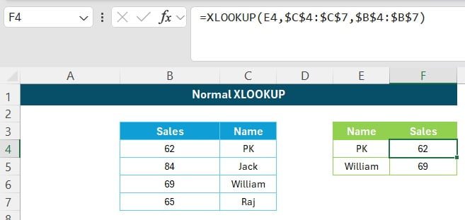
Let’s start with the basics. Suppose you have a dataset that lists the sales figures of different employees, and you need to retrieve the sales numbers based on their names. Here’s how you can do it:
Solution:
We can use the XLOOKUP function to find the sales for specific employees. Here’s the formula:
=XLOOKUP(E5, $C$4:$C$7, $B$4:$B$7)
In this formula:
E5 is the cell where the name you’re looking up is located.
$C$4:$C$7 is the range where the names are listed.
$B$4:$B$7 is the range where the corresponding sales figures are listed.
When you use this formula, Excel will return the sales number for the name specified in cell E5. For instance, if you look up “PK”, the function will return 62.
Example 2: Master XLOOKUP with Multiple Lookup Values
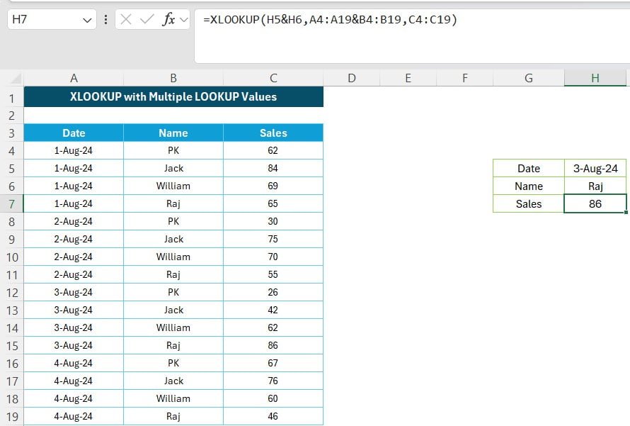
Now, let’s step it up a notch. What if you have a dataset with multiple entries for each name on different dates, and you want to retrieve sales figures for a specific date and name combination? XLOOKUP can handle that too!
Solution:
Here’s the formula that looks up sales based on both date and name:
=XLOOKUP(H5&H6,A4:A19&B4:B19,C4:C19)
In this formula:
H5 contains the date you’re looking up.
H6 contains the name.
- A4:A19&B4:B19 concatenates the date and name columns, which XLOOKUP will search through.
- C4:C19 contains the sales figures.
For example, if you’re looking for the sales on “3-Aug-24” for “Raj,” this formula will return 86.
Example 3: Finding the Last Occurrence with XLOOKUP
Sometimes, you need to find the last occurrence of a value in a dataset. With XLOOKUP, you can achieve this with ease.
Solution:
To find the last sale made by “Jack,” you can use the following formula:
=XLOOKUP(H6,B4:B19,C4:C19,,,-1)
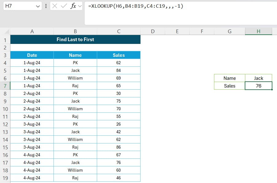
Here’s what’s happening:
The formula searches through the list backward (thanks to the -1 argument), ensuring that it returns the last occurrence of “Jack” in the list.
If you’re looking up “Jack,” XLOOKUP will return 76, the sales number from his last recorded sale.
Example 4: Finding the Last Sale with Latest Date
Just as you can find the last occurrence, you can also locate the first sale using the latest date in your dataset.
Solution:
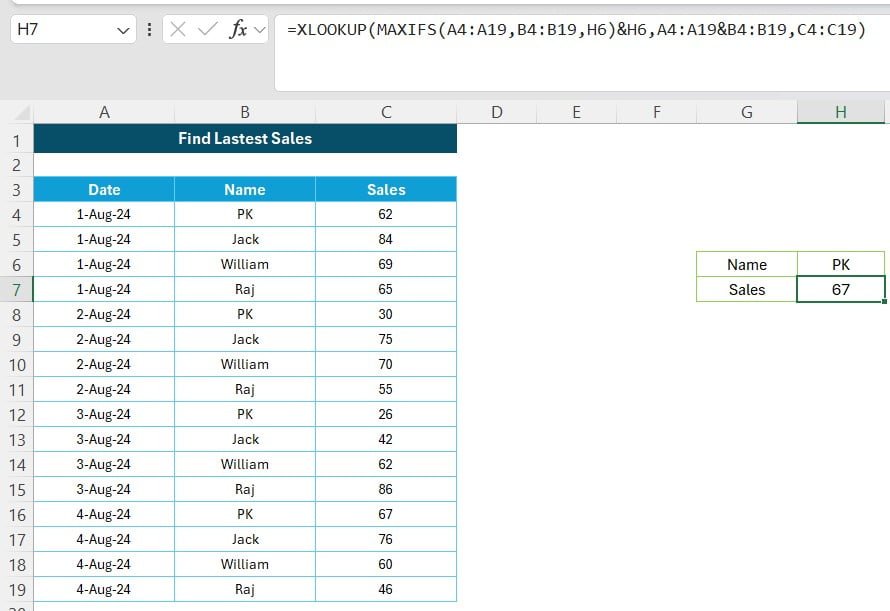
Use this formula to find the earliest sale for “PK”:
=XLOOKUP(MAXIFS(A4:A19, B4:B19, H6)&H6,A4:A19&B4:B19,C4:C19)
Example 5: Finding the First Sale with Earliest Date
Just as you can find the first occurrence, you can also locate the first sale using the earliest date in your dataset.
Solution:
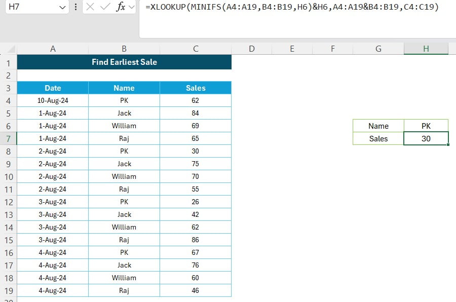
Use this formula to find the earliest sale for “PK”:
=XLOOKUP(MINIFS(A4:A19, B4:B19, H6)&H6,A4:A19&B4:B19,C4:C19)
Example 6: Error Handling in XLOOKUP
Errors can be frustrating, but XLOOKUP allows you to handle them gracefully by returning a custom message when a value is not found.
Solution:
Here’s a formula that returns “Not Found” if the name you’re looking up doesn’t exist in the dataset:

=XLOOKUP(H6, B4:B19, C4:C19,"Not Found")
For instance, if you search for a name that isn’t in the list, XLOOKUP will return “Not Found” instead of an error.
Example 7: Aging Bucket
XLOOKUP can help you to create the aging bucket on the basis of another table-
Solution:
Here’s how to categorize ages into buckets:
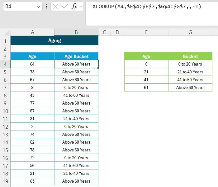
=XLOOKUP(A19, $F$4:$F$7,$G$4:$G$7,,-1)
This formula matches the ages in column A with the corresponding age buckets in columns F and G.
Example 8: Dynamic Results with XLOOKUP
XLOOKUP can also return dynamic results based on different criteria, making it a highly adaptable tool.
Solution:
To find dynamic results based on changing criteria:
=XLOOKUP(H6,CHOOSECOLS(A4:D18,MATCH(G6,A3:D3,0)),CHOOSECOLS(A4:D18,MATCH(G8,A3:D3,0)),"Not Found")

This formula allows you to search for values across different columns dynamically.
Example 9: Wildcard Character Match
Sometimes, you may need to match partial text strings. XLOOKUP supports wildcard character matches, making this easy.
Solution:
Here’s how to use wildcards:
=XLOOKUP(G6, A4:A18, B4:B18,2)

If you search for “10001*”, XLOOKUP will return the corresponding sales value.
Example 10: Regex Match in XLOOKUP
For more advanced matching, you can use regular expressions with XLOOKUP, giving you powerful control over your searches.
Solution:
To use regex:
=XLOOKUP(G6&"|"&I6, A4:A8, B4:B8,"Not Found",3)

This formula allows for complex searches that combine multiple criteria.
Note: This is a new feature and available only in beta version.
Wrapping Up
XLOOKUP is a game-changer in Excel, offering flexibility and power for a wide range of data lookup tasks. From simple lookups to complex data retrievals involving multiple criteria, XLOOKUP simplifies the process while improving accuracy and efficiency. Whether you’re new to Excel or a seasoned user, mastering XLOOKUP will undoubtedly enhance your productivity. Keep experimenting with different scenarios, and soon you’ll find that XLOOKUP is an indispensable tool in your Excel arsenal.
Visit our YouTube channel to learn step-by-step video tutorials
Watch the step-by-step video tutorial:
Click Here to download the Practice File

