In this video, we have explained how to create a Quick Weekly Attendance Template in Excel using New Check box feature in office 365 and Conditional formatting.
Follow the below given step to achieve this-
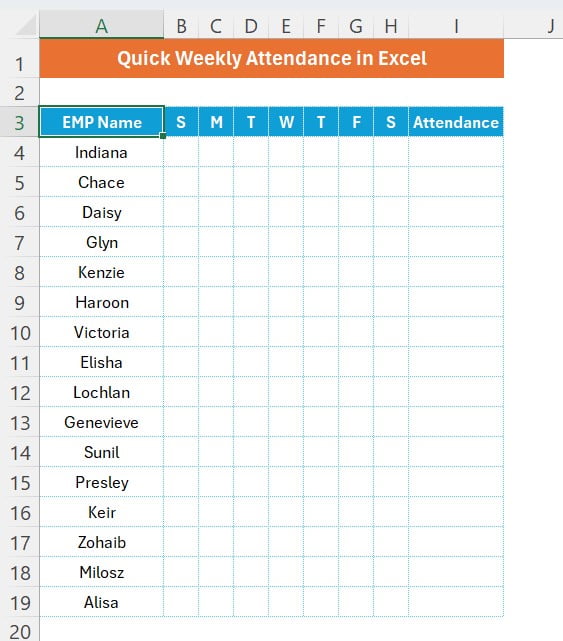
Put the headers:
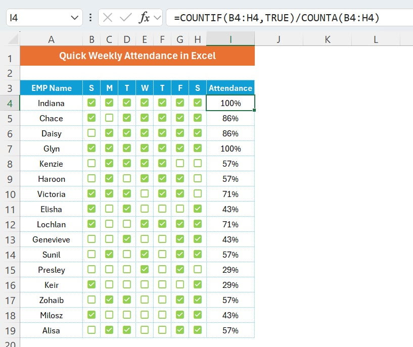
Add the headers first from Range A3 to I3 as given below
- Emp Name on A3
- First letter of the day as S, M, T, W, T, F and S on range B3 to H3
- Put “Attendance” on range I3
Enter Emp Names:
Put the Employee name on from range A4. We have put here Emp Name from range A4 to A19.
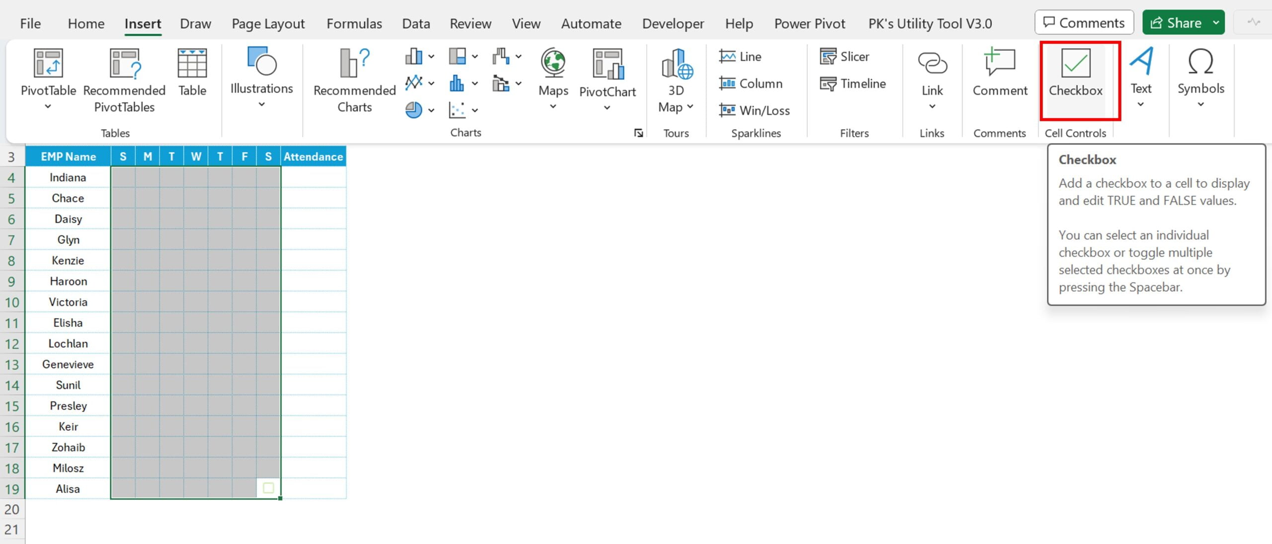
Insert check boxes:
- Select the range B4:H19
- Go to insert and insert the check box
- Take the font size as 8
- Reduce the column width as 2.5 or 3
- Take the font color as light green
Put the Attendance Formula:
- Put the formula on range I4 as “=COUNTIF(B4:H4,TRU/COUNTA(B4:H4)”
- Fill this down from I4 till I19
- change into percentage format using shortcut key Shift+Ctrl+5
Add Conditional Formatting Data Bar:
- Select the range I4:I19
- Press Alt +O+D to open the Conditional Formatting Rule Manager.
- Click on New Rule
- Select Format Style as “Data Bar”
- Select Minimum and Maximum Type as Number.
- Take Minimum Value as 0 and Maximum value as 1
- Select Gradient Fill in Fill.
- Choose Color as orange.
- Choose Solid Border in Border and Border color as Orange.
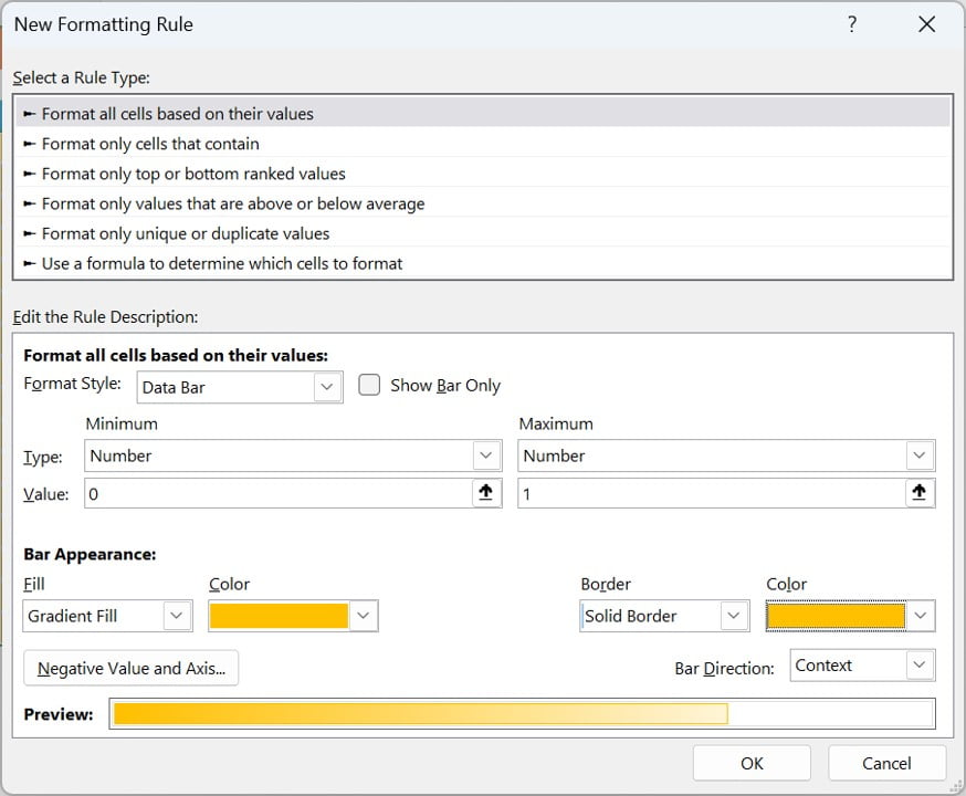
- Click on OK and Apply the Rule.
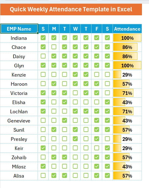
Our Quick Weekly Attendance Template in Excel is ready to use.
Visit our YouTube channel to learn step-by-step video tutorials

