When analyzing data in Excel, ranking values can be incredibly useful to understand the position of each item relative to others. In this blog post, we’ll break down how to use the RANK function in Excel by walking through a clear example. Whether you’re a student calculating grades or a professional analyzing sales data, this function will quickly become one of your favorite’s!
What Does the RANK Function Do in Excel?

The RANK function in Excel is designed to return the rank of a number in a list of numbers. Essentially, it tells you how a specific number compares to others—whether it’s the highest, lowest, or somewhere in between.
Example Scenario
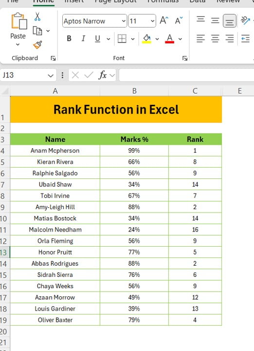
Let’s take an example to make this easier to understand. We have a dataset that contains the names of students, their percentage marks, and the rank we want to calculate. We’ll show you how to determine each student’s rank based on their marks using the Rank Function in Excel.
Step-by-Step Guide to Using the RANK Function
To find the ranks of the students based on their percentage marks, follow these steps:
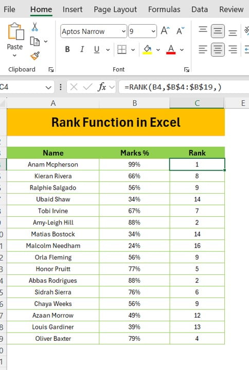
- Select the Cell: First, click on the cell where you want the rank to appear. In our case, we’ll start with the rank for Annam McPhersons.
- Enter the Formula: In the selected cell, enter the following formula:
=RANK (B2, $B$2: $B$17)

Let’s break down this formula:
- B2 is the cell that contains Annam’s percentage.
- $B$2: $B$17 is the range that includes all the marks. We use the dollar signs to lock the range so that it doesn’t change when the formula is copied to other cells.
- Copy the Formula: After you’ve entered the formula for the first cell, you can copy it down for the other students. Excel will automatically adjust the reference to the next student’s marks.
- Review the Ranks: Once the formula has been applied, you’ll see the ranks for all students based on their marks.
What About Ties?
One thing to note is that when two or more students have the same marks, Excel will assign the same rank to all of them. In our example, Amy-Leigh Hill and Abbas Rodrigues both scored 88%, so they share the same rank (2). Similarly, Ralphie, Orla, and Chaya all have 56%, and they’re ranked 9.
Why Use the RANK Function?
Now that we’ve walked through how to use the RANK function, let’s explore why it’s so valuable:
- Efficient: When you have a large dataset, manually calculating ranks would be time-consuming. The RANK function does the work for you.
- Flexible: You can easily adjust the ranking to be in ascending or descending order by modifying the formula.
- Insightful: Ranking provides a quick snapshot of performance, whether you’re dealing with academic scores or business data.
Conclusion
As you can see, the RANK function in Excel is a powerful tool for comparing and organizing data. With just a simple formula, you can rank numbers efficiently and accurately. Whether you’re working on student marks, sales figures, or any other type of data, this function helps streamline your analysis.
Feel free to watch the video tutorial linked below for a step-by-step visual guide!
Let us know in the comments if you’ve found this helpful, and don’t forget to share it with others who might benefit from learning this handy Excel feature!
Visit our YouTube channel to learn step-by-step video tutorials
View this post on Instagram
Click hare to download the practice file


