Have you ever wondered how to calculate the interest rate required for an investment to grow from its present value to a future value over a specified number of periods? Excel’s RRI function can help you with that! In this post, we’ll walk through how to use the RRI function in Excel using a real example, making it easy to understand and apply to your own data. By the end of this guide, you’ll feel confident using this powerful function to calculate compound interest rates.
What Is the RRI Function in Excel?
The RRI (Rate of Return for an Investment) function in Excel calculates the equivalent annual interest rate required for an investment to grow from its present value to its future value over a specified number of periods. Essentially, it helps you determine how fast your investment needs to grow to achieve your financial goals.
The syntax for the RRI function is as follows:
=RRI (NPER, PV, FV)
- NPER: The number of periods (e.g., months, years).
- PV: The present value of the investment.
- FV: The future value of the investment.
Now that we know the basics, let’s jump into a practical example to see how this works in real life.
Example Data: Investment Growth Over Time
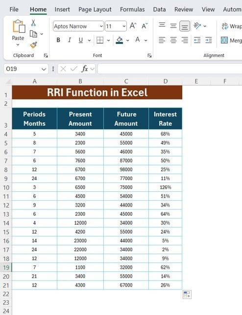
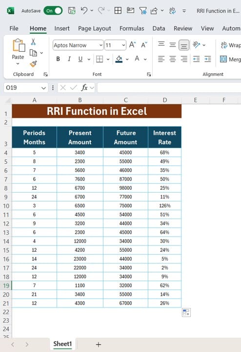
We have a dataset that represents the number of periods, present amounts, and future amounts for various investments. The goal is to calculate the interest rate needed for each investment to reach its future value using the RRI function.
Applying the RRI Function in Excel
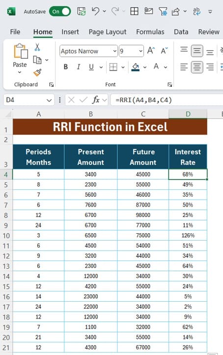
To calculate the interest rate required for each investment, we’ll use the RRI function. The formula we use is simple:
=RRI (A4, B4, C4)
This formula will take the number of periods in column A, the present value from column B, and the future value from column C to calculate the required interest rate.
For example, let’s calculate the interest rate for the first row:
- Periods (Months): 5
- Present Amount: 3,400
- Future Amount: 45,000
Using the formula =RRI (5, 3400, 45000), we get an interest rate of 68%. This means that for an investment of $3,400 to grow to $45,000 in 5 months, the interest rate needs to be 68%.
Step-by-Step Process to Use the RRI Function
Let’s break this down into easy steps:
- Select the cell where you want the result.
- Enter the formula: =RRI(A4, B4, C4) (replace the cell references with the relevant cells from your dataset).
- Press Enter, and Excel will return the interest rate for that investment.
Practical Tips When Using RRI Function
Here are a few tips to keep in mind while using the RRI function:
- Consistency in Periods: Ensure that the periods you use (e.g., months, years) are consistent throughout the data. If one investment uses months and other uses years, the results won’t be accurate.
- Negative Values: Avoid using negative values for present or future amounts. The RRI function assumes the values are positive investments or savings.
- Interest Rate Format: Excel may return the result as a decimal. To display it as a percentage, you can format the cell as a percentage by right-clicking on it and selecting Format Cells.
Conclusion
The RRI function in Excel is an excellent tool for calculating the interest rate required for an investment to reach its future value. Whether you’re managing personal finances, investment portfolios, or even business forecasting, this function helps you quickly and accurately determine the growth rate needed.
By applying the RRI formula to your data, you can easily calculate the rate of return for any investment scenario. So go ahead, try it on your own datasets, and let Excel do the hard work for you!
Visit our YouTube channel to learn step-by-step video tutorials
View this post on Instagram
Click hare to download the practice file
