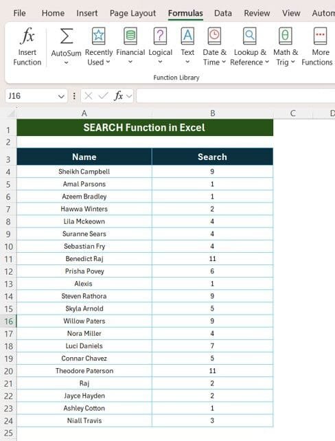
Are you ready to learn a new Excel skill that will make working with text so much easier? Today, we’re diving into the SEARCH function in Excel, a great tool that helps you find text within larger pieces of data. Let’s go over how this function works, step by step, so you can use it effectively and make your data analysis tasks a breeze SEARCH Function in Excel.
What Does the SEARCH Function Do in Excel?
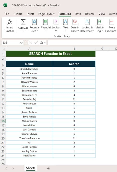
First off, let’s understand what the SEARCH function is all about. Imagine you have a long list of text or names, and you’re trying to locate a specific letter or word within that list. That’s exactly what the SEARCH function helps with! It scans each cell, finds where a certain letter or word appears, and tells you about its position within the text. This can be super helpful if you’re working with names, codes, or any text-heavy data.
The formula for the SEARCH function looks like this:
=SEARCH (find text, within text, [start_ Num])
Here’s a quick breakdown of each part:
- find text: The text (like a letter or word) that you want to look for.
- within text: The cell or text where you want to search for your specified text.
- start_ Num: This is optional. It’s the position where you want the search to start. If you skip it, Excel will start from the beginning.
Let’s try it out with a real example so you can see it in action!
This table has two columns:
- Name (in cells A3): Here, we’ve listed different names.
- Search (in cells B3): This is where we’ll show the position of the letter “A” for each name.
How to Use the SEARCH Function to Find “A”
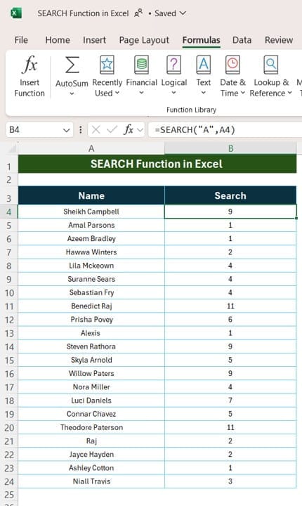
To locate the letter “A” within each name, we’ll use the SEARCH function. Here’s the exact formula to type into Excel:
=SEARCH (“A”, A4)
Breaking Down the Formula:
- We’re searching for “A” within each name.
- A4 is the cell containing the name we want to analyze.
Once you type this formula into a cell in the Search column, Excel will show you the position of “A” in the name. For example:
- For “Amal Parsons”, it shows 1, because “A” is at the beginning of the name.
- For “Sheikh Campbell”, it shows 9, as the first “A” appears in the ninth position.
Step-by-Step Guide: Using the SEARCH Function
Ready to try it yourself? Here’s a quick, easy guide to getting this function to work on your data:
- Pick a cell in the Search column where you want to place the result.
- Type the formula: Start with =SEARCH (“A”, A4). Replace A4 with the cell that contains the name.
- Press Enter: Excel will instantly return the position of “A” for that name.
- Copy the formula down the column: Simply drag the formula to apply it to other cells in the Search column.
As you fill in the formula for each cell, Excel will calculate the position of “A” for every name in the list.
Why Use the SEARCH Function?
There are plenty of reasons to start using the SEARCH function in Excel! Here are just a few:
- Flexible Text Matching: Quickly find specific letters or words within larger pieces of text.
- Easy Data Filtering: Filter or categorize data based on the presence of certain text.
- Great for Organizing Data: Helps you manage and organize text-heavy data efficiently.
Quick Tips for Using the SEARCH Function
Before we wrap up, here are a few quick tips to make the SEARCH function even easier to use:
- Case Insensitive: Unlike the FIND function, SEARCH doesn’t care about uppercase or lowercase letters. It treats “A” and “a” as the same.
- Error Handling: If the text you’re searching for isn’t there, Excel returns an error. To avoid this, use IFERROR to handle missing text gracefully.
Visit our YouTube channel to learn step-by-step video tutorials
View this post on Instagram
