Introduction
In the fast-paced world of data analysis, efficiency and flexibility are key. That’s why in our latest video, “SUM + CHOOSECOLS Function for Dynamic Total” we delve into a game-changing Excel formula that streamlines the process of summing up sales data dynamically. This guide is designed to complement the video, making the leap from screen to actionable knowledge smoother and more intuitive.
The Challenge: Dynamic Data Summation
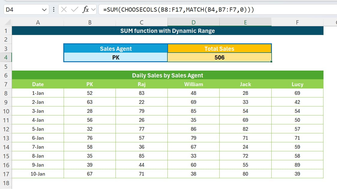
Imagine you’re analyzing daily sales data by sales agent. You’re working with a dataset spanning from range A7:F17, with headers in A7:F7 indicating the date and sales agents’ names (PK, Raj, William, Jack, and Lucy). Your goal? To dynamically calculate the total sales for a selected agent without manually adjusting your formulas every time the selection changes.
The Solution: SUM + CHOOSECOLS function
Enter the powerful combination of the SUM function with CHOOSECOLS. The formula we showcased in our video is:
=SUM(CHOOSECOLS(B8:F17,MATCH(B4,B7:F7,0)))

But what makes this formula a game-changer? Let’s break it down:
Understanding the Formula Components
- SUM Function: A staple in Excel, used here to calculate the total sum of a range of cells.
- CHOOSECOLS Function: This function is the star of the show, allowing us to dynamically select columns from a specified range based on the criteria we define.
- MATCH Function: It searches for the selected sales agent’s name in the headers (B7:F7) and returns the position of that name within the range. This position number is then used by CHOOSECOLS to select the correct column.
How It Works Together
- Selection via Dropdown: You select a sales agent from a dropdown list in B4. This could be any of the agents: PK, Raj, William, Jack, or Lucy.
- Dynamic Column Selection: The MATCH function finds the position of the selected agent’s name in the header row (B7:F7).
- Summation of Selected Data: CHOOSECOLS function is using the position number returned by MATCH to get the correct column from B8:F17. Finally, SUM adds up the values in this dynamically selected column.
Why This Matters
This isn’t just about making calculations easier (though it certainly does that!). It’s about transforming the way you approach data analysis. Suddenly, what used to be a chore becomes a swift, seamless process, leaving you more time to dive into what the numbers are really saying.
Wrapping It Up: A Step Towards Smarter Analysis
The journey from a powerful video demonstration to an engaging, easy-to-follow written guide is all about making sure you’ve got the tools and understanding to work smarter, not harder. With this dynamic duo of SUM and CHOOSECOLS, you’re not just crunching numbers; you’re setting the stage for deeper insights and more efficient data handling.
Visit our YouTube channel to learn step-by-step video tutorials
Watch the step-by-step video tutorial:
Click here to download the practice file


