Have you ever wondered how to quickly sum data from multiple columns in Excel? If so, you’re in the right place! In this guide, I’m going to show you exactly how to use the SUM+VLOOKUP Formula in Excel. Whether you’re new to Excel or have been using it for years, this trick will make your work much easier.
Let’s dive in and explore how to use this powerful formula combination!
What is the SUM + VLOOKUP Formula in Excel?
Before we jump into the details, let’s break it down. The SUM + VLOOKUP formula is a simple yet powerful tool that helps you find specific data and then sum it across multiple columns. You’ll often use this when you want to quickly add up values, like sales or expenses, from a large dataset SUM+VLOOKUP Formula.
Now, here’s why you’d want to use it:
Why Use SUM + VLOOKUP?
- It saves time: You don’t have to manually search and sum the values.
- It reduces errors: With just one formula, you can sum data accurately.
- It’s flexible: You can sum data from multiple columns all at once.
Sounds useful, right? Let’s go through an example together so you can see how it works.
Example: SUM + VLOOKUP for Monthly Sales Data
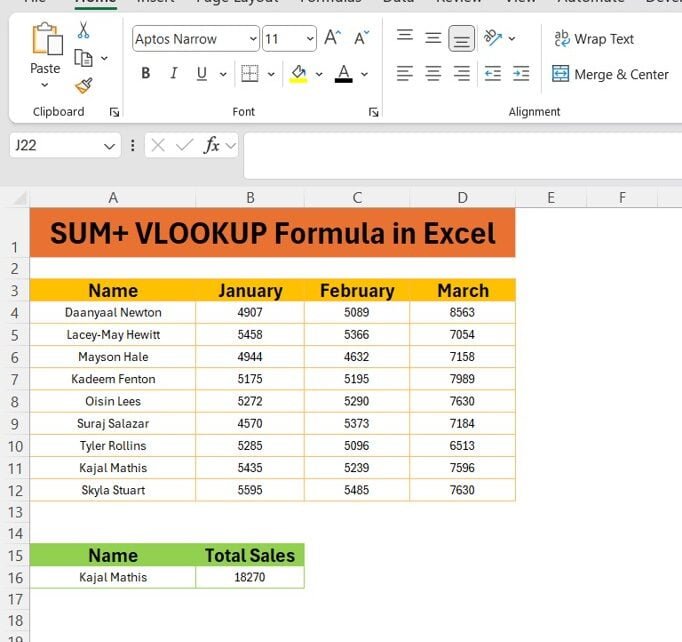
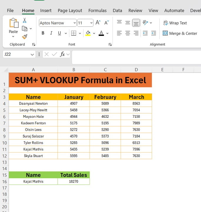
Imagine you’re managing sales data for your team, and you need to find the total sales for each employee over three months (January, February, and March). You have the following data:
Your goal is to find the total sales for Kajal Mathis across all three months.
Step-by-Step: How to Use SUM + VLOOKUP
Let’s walk through the steps together:
- Set up your data: Make sure your data is in an easy-to-read table. You’ll have names in the first column and the sales figures in the next three columns (January, February, and March).
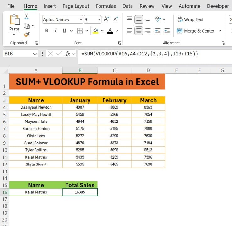
- Enter the formula: Now, we’re going to use the SUM + VLOOKUP formula to find and add up the sales for Kajal Mathis. In any blank cell, type the following formula:
=SUM(VLOOKUP(A16, A3:D11, {2,3,4}, 0))
Let me explain what’s happening here:
- A16: This is the cell where you’ll type the name you’re looking for (e.g., Kajal Mathis).
- A3: This is the range of your data (where columns A to D contain the names and sales data).
- {2,3,4}: These are the column numbers for January, February, and March. We’re telling Excel to look in these columns.
- 0: This ensures an exact match for the name you’re looking for.
- Press Enter: Once you press Enter, Excel will find Kajal Mathis in the data and add up her sales for January, February, and March.
The Result
After you hit Enter, Excel will show you the total sales for Kajal Mathis across those three months:
Name Total Sales
Kajal Mathis 18,270
That’s it! In just one formula, you’ve summed the data from three different columns.
Why This Formula is So Useful
You might be wondering why this formula is such a big deal. Well, here are a few reasons why it’s going to make your life easier:
- Saves Time: You don’t need to manually sum data from different columns—Excel does it for you.
- Reduces Errors: Manually adding numbers is prone to mistakes. This formula ensures everything is accurate.
- Simplifies Your Work: Instead of using multiple formulas, you can do everything in one step.
Final Thoughts
The SUM + VLOOKUP formula is a game-changer when it comes to working with data in Excel. It’s quick, reliable, and will save you a ton of time. If you deal with large datasets or need to sum values from different columns regularly, this formula is your new best friend.
So, give it a try in your next Excel project! You’ll be amazed at how much time and effort it saves you.
Visit our YouTube channel to learn step-by-step video tutorials
View this post on Instagram
Click hare to download the practice file
