Have you ever found yourself lost in a large data set, trying to match values across columns? Excel’s VLOOKUP function is here to save the day! In this blog post, we’ll explore some easy hacks using the VLOOKUP formula to pull information effortlessly. We’ll not only walk you through the steps but also provide a real-world example that will help you master this popular Excel tool in no time!
What is VLOOKUP in Excel?
The VLOOKUP function is a powerful tool that searches for a value in the first column of a data range and returns a value in the same row from another column. It’s ideal when working with structured data like grades, percentages, product codes, or customer details.
Example Scenario: Extracting Names, Percentages, and Grades
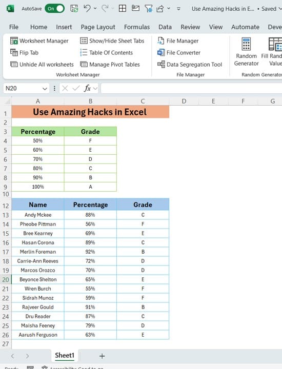
In our example, we are working with a list of students and their corresponding percentages and grades. Below, we have three columns in the dataset:
- Names in Column A
- Percentages in Column B
- Grades in Column C
The goal here is to use VLOOKUP to easily retrieve a student’s grade based on their percentage.
Data Setup in Excel
To get started, here’s how we’ve structured our data:
- Column A (Names): Located in A12
- Column B (Percentages): Located in B12
- Column C (Grades): Located in C12
How to Use VLOOKUP to Retrieve Grades
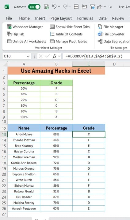
Let’s say we want to quickly pull the grade for a student based on their percentage using the VLOOKUP formula. Follow these steps to see the magic unfold!
- Select the cell where you want the grade to appear (e.g., C13).
- Use the formula:
=VLOOKUP (B13, $A$4: $B$9, 2)
- B13: The percentage we are looking up.
- $A$4: $B$9: The range containing percentages and grades.
- 2: The column index from which we want to return the value (in this case, the grade column).
- Drag the formula down for all students to quickly fetch their grades based on their percentages.
Why Use VLOOKUP for This Task?
- Quick and Easy – With a simple formula, you can retrieve data in seconds!
- Eliminates Manual Effort – No need to search rows manually; VLOOKUP does the job for you.
- Dynamic Updates – If your data changes, the results update automatically with VLOOKUP.
Pro Tip: Use Absolute References for Reliable Results
Notice how we used $A$4: $B$9 in the formula? The dollar signs ensure that the range stays fixed even when you drag the formula to other cells. Without it, the reference would shift, leading to incorrect results.
Common VLOOKUP Errors and How to Avoid Them
- #N/A Error – This happens when the lookup value isn’t found in the first column of the range.
- Solution: Double-check your data to ensure the value exists.
- #REF! Error – This occurs if the column index you provide is greater than the number of columns in the range.
- Solution: Ensure the column index matches the structure of your data.
Wrapping It Up
With the VLOOKUP function, matching data in Excel becomes a breeze! Whether you’re handling grades, products, or customer details, VLOOKUP can save you hours of manual work. Don’t just stop here—explore other Excel functions and combine them with VLOOKUP for even more efficiency!
If you found these tips helpful, check out our YouTube video on the same topic for a visual walk-through. Click the link below and level up your Excel game today!
Visit our YouTube channel to learn step-by-step video tutorials
View this post on Instagram
Click hare to download the practice file

